VINS-Mono 논문 번역 & 공부 (1)

2022. 1. 19.

#SLAM #VINS-Mono

Related Work 부분은 나중에 추가할 예정입니다.
Section.V Initialization의 내용까지 정리하였습니다.
코드 Github 논문 PDF

Introduction

VINS-Mono는 다음과 같은 특징을 가지고 있습니다.

robust initialization procedure that is able to bootstrap the system from unknown initial states.
tightly coupled, optimization-based monocular VIO with camera–IMU extrinsic calibration and IMU bias correction.
online relocalization and four degrees-of-freedom (DOF) global pose graph optimization.
pose graph reuse that can save, load, and merge multiple local pose graphs.

Overview

Structure

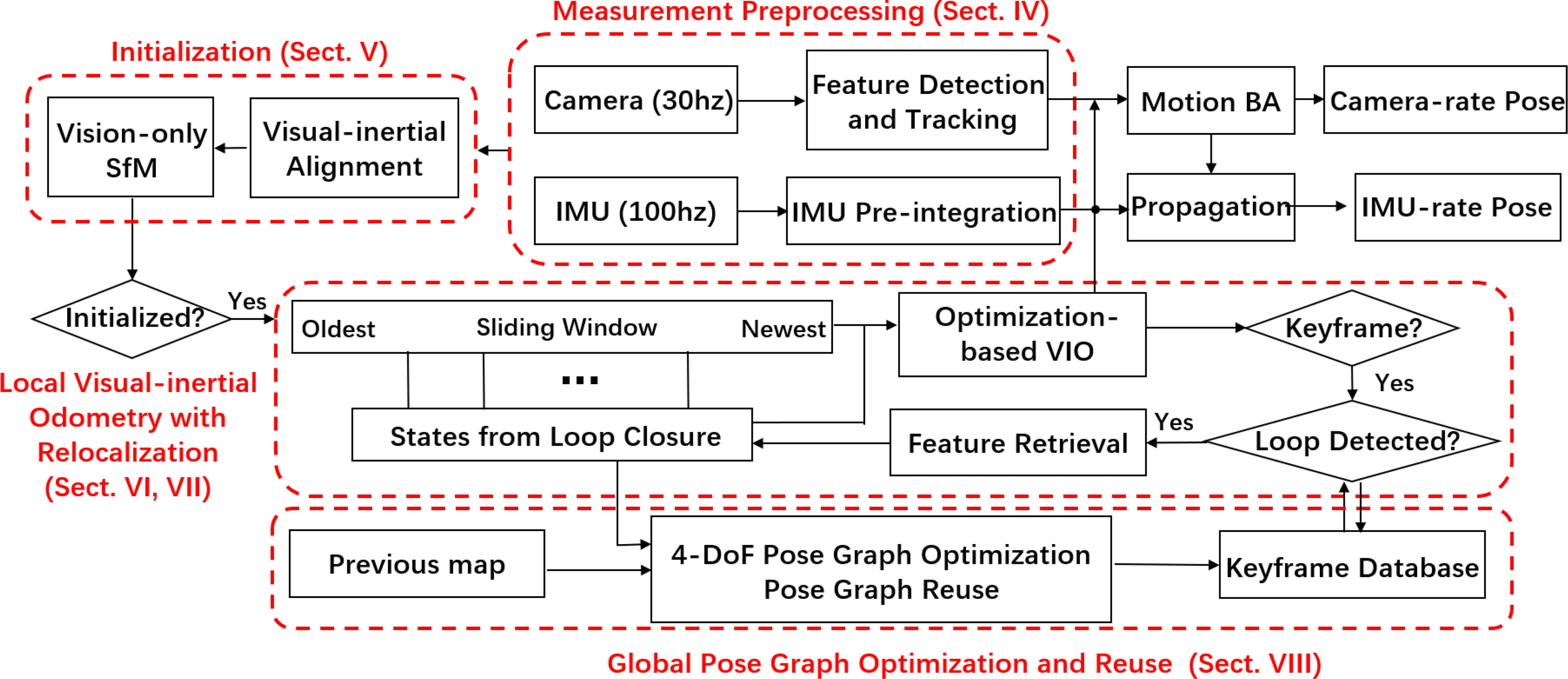
monocular visual-inertial state estimator의 구조입니다.

시스템은 measurement preprocessing으로 시작합니다. (Section IV)

feature가 extract and tracked되고, 두 프레임 사이의 IMU 측정값이 preintergrate 됩니다.

Initialization 과정은 필요한 모든 값들을 제공합니다. (Section V)

for bootstrapping the subsequent nonlinear optimization-based VIO.
pose, velocity, gravity vector, gyroscope bias, and three-dimensional (3-D) feature location.

The VIO (Section VI) with relocalization (Section VII) 모듈

preintegrated IMU measurements와 feature observations를 tightly 통합합니다.

마지막으로 pose graph optimization 모듈. (Section VIII)

takes in geometrically verified relocalization results.
perform global optimization to eliminate the drift.
also achieves the pose graph reuse.

The VIO와 pose graph optimization 모듈은 각각의 thread에서 동시에 동작합니다.

Notation and Frame Definitions

$(\cdot)^w$ : world frame, 중력의 방향은 world frame의 z축과 align되어 있습니다.
$(\cdot)^b$ : body frame (IMU frame)
$(\cdot)^c$ : camera frame
$\mathbf{R}$ : rotation matrix
$\mathbf{q}$ : Hamilton quaternion
- 주로 state vector에 사용
- 3D vector의 편한 회전 연산을 위해서 사용됨
$\mathbf{q}_{b}^{w}, \mathbf{p}_{b}^{w}$ : rotation and translation from the body frame to the world frame
$b_k$ : the body frame while taking the $k$ th image
$c_k$ : the camera frame while taking the $k$ th image.
$\otimes$ : represents the multiplication operation between two quaternions
$\mathbf{g}^w = [0,0,g]^T$ : the gravity vector in the world frame
$\hat{(\cdot)}$ : the noisy measurement or estimation of a certain quantity

Measurement Preprocessing

IMU와 Monocular 이미지의 preprocessing에 대해 설명하겠습니다.

Visual measurements
- 연속된 두 프레임 사이의 features를 추적하고 마지막 프레임에서 새로운 feature를 detect합니다.
IMU measurements
- we preintegrate them between two consecutive frames.

Vision Processing Front End

새로운 이미지에대해 existing features가 KLT sparse optical flow algorithm[31]을 이용해 tracking됩니다. 동시에 각각의 이미지가 최소 100~300개의 feature를 가질 수 있도록 새로운 corner features가 detect[32] 됩니다. detector는 인접한 2개의 feature사이의 최소 픽셀 거리를 설정하여 균일한 feature distribution을 가질 수 있도록 합니다.

이후 2D features는

undistorted된 후 (왜곡 보정)
outlier rejection (performed using RANSAC with a fundamental matrix model) [33]
unit sphere에 project됩니다.

[31] B. D. Lucas and T. Kanade, “An iterative image registration technique with an application to stereo vision,” in Proc. Int. Joint Conf. Artif. Intell., Vancouver, Canada, Aug. 1981, pp. 24–28.

[32] J. Shi and C. Tomasi, “Good features to track,” in Proc. IEEE Int. Conf. Pattern Recog., 1994, pp. 593–600.

[33] R. Hartley and A. Zisserman, Multiple View Geometry in Computer Vision. Cambridge, U.K.: Cambridge Univ. Press, 2003.

Keyframes 또한 이 단계에서 선택됩니다. Keyframes selection을 위한 2개의 기준은 다음과 같습니다.

이전 keyframe과의 평균 parallex
- 만약에 traking된 features가 current frame과 latest프레임 사이에 있고, 평균 parallex가 특정 threshold값을 넘으면, frame을 새로운 keyframe으로 간주합니다.
- 만약 회전이벤트만 있을 경우 triangluate이 불가능하기 때문에 gyroscope measurements를 적분하여 parallex계산에 사용합니다.
  - 이 계산은 오직 keyframe selection에만 사용되며, gyroscope measurements의 noise가 커도 가장 최적이 아닌 keyframe selection될 뿐 전체 퀄리티에 바로 영향을 주지는 않습니다.
Tracking quality
- 만약 tracking된 features의 수가 특정 threshold보다 작아지면, frame을 새로운 keyframe으로 간주합니다.
- 이것은 feature tracking을 완전히 실패했을 때를 위해서임

IMU Preintegration

[19]와 [24]의 방법을 이용한 the handling of IMU biases를 포함하여 우리의 이전 연구인 continuous-time quaternion-based derivation of IMU preintegration을 따릅니다.

IMU preintegration의 수치적 결과는 [19], [24]와 거의 동일합니다. 차이점은 다른 derivation을 사용한다는 것입니다.

그래서 우리는 간단한 introduction만 하겠습니다.

[19] C. Forster, L. Carlone, F. Dellaert, and D. Scaramuzza, “On-manifold preintegration for real-time visual–inertial odometry,” IEEE Trans. Robot., vol. 33, no. 1, pp. 1–21, Feb. 2017.

[24] C. Forster, L. Carlone, F. Dellaert, and D. Scaramuzza, “IMU preintegration on manifold for efficient visual-inertial maximum-a-posteriori estimation,” in Proc. Robot., Sci. Syst., Rome, Italy, Jul. 2015.

quaternion-based derivation에 대한 자세한 내용은 Appendix A에서 확인할 수 있습니다. IMU Preintegration

IMU Noise and Bias

body frame에서 측정된 IMU measurements는 플랫폼(로봇)의 dynamics와 중력의 반대로 가해지는 힘의 결합입니다. 그리고 acceleration bias $\mathbf{b}_a$ , gyroscope bias $\mathbf{b}_w$ , additive noise에 영향을 받습니다.

accelerometer와 gyroscope의 raw measurements $\hat{\bf{a}}, \hat{\boldsymbol{\omega}}$ 는 다음과 같이 주어집니다.

\begin{equation} \begin{align*} \hat{\mathbf{a}}_t &= \mathbf{a}_t + \mathbf{b}_{a_t} + \mathbf{R}^t_w\mathbf{g}^w + \mathbf{n}_a \\ \hat{\boldsymbol{\omega}}_t &= \boldsymbol{\omega}_t + \mathbf{b}_{\omega_t} + \mathbf{n}_\omega \end{align*} \end{equation}

additive noise가 Gaussian white noise라고 가정합니다. $\mathbf{n}_a \sim \mathcal{N}(\mathbf{0}, \boldsymbol{\sigma}^2_{a}),\ \mathbf{n}_\omega \sim \mathcal{N}(\mathbf{0}, \boldsymbol{\sigma}^2_\omega)$

Acceleration bias와 gyroscope bias의 모델은 random walk이고, derivatives는 Gaussian white noise입니다. $\mathbf{n}_{b_a} \sim \mathcal{N}(\mathbf{0}, \boldsymbol{\sigma}^2_{b_a}), \ \mathbf{n}_{b_\omega} \sim \mathcal{N}(\mathbf{0}, \boldsymbol{\sigma}^2_{b_\omega})$

\begin{equation} \dot{\mathbf{b}}_{a_t} = \mathbf{n}_{b_a} \quad \dot{\mathbf{b}}_{\omega_t} = \mathbf{n}_{b_\omega} \end{equation}

Preintegration

연속된 두개의 body frame $b_k, b_{k+1}$ 에 대하여, $[t_k, t_{k+1}]$ 시간 동안의 IMU 측정값이 존재한다.

주어진 bias estimation을 통해 우리는 local frame $b_k$ 에 다음과 같이 통합합니다.

\begin{equation} \begin{align*} \boldsymbol{\alpha}_{b_{k+1}}^{b_k} &= \int\int_{t\in [t_k,t_{k+1}]} {\mathbf{R}_{t}^{b_k}(\hat{\mathbf{a}}_t - \mathbf{b}_{a_t})dt^2} \\ \boldsymbol{\beta}_{b_{k+1}}^{b_k} &= \int_{t\in [t_k,t_{k+1}]} {\mathbf{R}_{t}^{b_k}(\hat{\mathbf{a}}_t - \mathbf{b}_{a_t})dt} \\ \boldsymbol{\gamma}_{b_{k+1}}^{b_k} &= \int_{t\in [t_k,t_{k+1}]} {\frac{1}{2}\boldsymbol{\Omega}(\hat{\boldsymbol{\omega}}_t - \mathbf{b}_{\omega_t})\gamma_{t}^{b_k}dt} \end{align*} \end{equation}

where

\begin{equation} \boldsymbol{\Omega}(\boldsymbol{\omega}) = \begin{bmatrix} -\lfloor\boldsymbol{\omega}\rfloor_\times & -\boldsymbol{\omega} \\ -\boldsymbol{\omega}^T & 0 \end{bmatrix}, \lfloor\boldsymbol{\omega}\rfloor_\times = \begin{bmatrix} 0 & -\omega_z & \omega_y \\ \omega_z & 0 & -\omega_x \\ -\omega_y& \omega_x & 0 \\ \end{bmatrix} \end{equation}

$\boldsymbol{\alpha}, \boldsymbol{\beta}, \boldsymbol{\gamma}$ 에 대한 covariance $P_{b_{K+1}}^{b_k}$ also propagates accordingly.

$b_k$ 를 bias가 주어진 reference로 이용하여 preintegration term $(3)$ 이 IMU 측정 값만을 통해 구할 수 있다는 것을 알 수 있습니다.

Bias Correction

bias 추정값이 조금 변경된다면 다음과 같은 1차 근사를 통해 $\boldsymbol{\alpha}_{b_{k+1}}^{b_k}, \boldsymbol{\beta}_{b_{k+1}}^{b_k}, \boldsymbol{\gamma}_{b_{k+1}}^{b_k}$ 를 적용합니다.

\begin{equation} \begin{align*} \boldsymbol{\alpha}_{b_{k+1}}^{b_k} &\approx \hat{\boldsymbol{\alpha}}_{b_{k+1}}^{b_k} + \mathbf{J}_{b_a}^{\alpha} \delta \mathbf{b}_{a_k} + \mathbf{J}_{b_\omega}^{\alpha} \delta \mathbf{b}_{\omega_k} \\ \boldsymbol{\beta}_{b_{k+1}}^{b_k} &\approx \hat{\boldsymbol{\beta}}_{b_{k+1}}^{b_k} + \mathbf{J}_{b_a}^{\beta} \delta \mathbf{b}_{a_k} + \mathbf{J}_{b_\omega}^{\beta} \delta \mathbf{b}_{\omega_k} \\ \boldsymbol{\gamma}_{b_{k+1}}^{b_k} &\approx \hat{\boldsymbol{\gamma}}_{b_{k+1}}^{b_k} \otimes \begin{bmatrix} 1 \\ \frac{1}{2} \mathbf{J}_{b_\omega}^{\gamma} \delta \mathbf{b}_{\omega_k} \end{bmatrix} \end{align*} \end{equation}

만약 bias가 많이 변한다면 새로운 bias 추정을 하고 repropagation합니다.

이런 방법은 IMU 측정값에 대한 propagate을 반복적으로 하지 않기 때문에 optimization-based algorithms을 사용할 때 컴퓨팅 리소스를 상당히 절약합니다.

Estimator Initialization

Monocular tightly coupled VIO는 정확한 initial guess를 요구하는 nonlinear 시스템입니다. IMU preintegration을 vision-only structure와 loosely align하여 우리는 필요한 initial value를 얻습니다.

Vision-Only SfM in Sliding Window

Initialization 과정은 up-to-scale camera poses와 feature positions 그래프를 estimate하기 위해 vision-only SfM으로 시작합니다.

우리는 제한된 컴퓨터의 성능을 생각하여 몇 개의 frame들을 sliding window안에 유지합니다.

먼저, 우리는 마지막 frame과 모든 이전 frame들 사이에 있는 feature correspondences를 체크합니다. 만약에 마지막 frame과 sliding window안의 다른 frame사이에서 안정적인 feature tracking(적어도 30개 이상 tracking)을 할 수 있고, 충분한 parallex(20 pixels 이상)가 있다면, 우리는 5-point algorithm[34]을 이용하여 두 frame사이의 relative rotation과 up-to-scale translation 정보를 얻을 수 있습니다.

[34] D. Nister, “An efficient solution to the five-point relative pose problem,” IEEE Trans. Pattern Anal. Mach. Intell., vol. 26, no. 6, pp. 756–770, Jun. 2004.

다음으로 임의의 scale을 설정하고 두 프레임에서 찾은 모든 feature들을 triangulate합니다. 이 triangulate된 feature들을 기반으로 다른 모든 frame에서의 pose를 estimate하기 위한 perspectiven-point (PnP) method[35]가 수행됩니다.

[35] V. Lepetit, F. Moreno-Noguer, and P. Fua, “EPnP: An accurate O(n) solution to the PnP problem,” Int. J. Comput. Vis., vol. 81, no. 2, pp. 155–166, 2009.

마지막으로 모든 feature observations에 대한 total reprojection error를 최소화하기위해 global full bundle adjustment[36]가 수행됩니다.

[36] B. Triggs, P. F. McLauchlan, R. I. Hartley, and A. W. Fitzgibbon, “Bundle adjustment: A modern synthesis,” in Proc. Int. Workshop Vis. Algorithms, 1999, pp. 298–372.

우리는 아직 world frame에 대한 정보가 없기 때문에 모든 SfM은 첫번째 카메라 frame $(\cdot)^{c_0}$ 을 기준으로 합니다. 모든 frame pose $(\bar{\mathbf{p}}_{c_k}^{c_0}, \mathbf{q}_{c_k}^{c_0})$ 와 feature position는 $(\cdot)^{c_0}$ 에 따라 표현됩니다. 주어진 camera와 IMU사이의 extrinsic parameter $(\mathbf {p}^b_c, \mathbf {q}^b_c)$ 를 이용해 모든 pose들을 camera frame에서 body frame으로 다음과 같이 변환할 수 있습니다.

\begin{equation} \begin{aligned} \mathbf {q}^{c_0}_{b_k} &= \mathbf {q}^{c_0}_{c_k} \otimes {(\mathbf {q}^b_c)}^{-1} \\ s\bar{\mathbf {p}}^{c_0}_{b_k} &= s\bar{\mathbf {p}}^{c_0}_{c_k} - \mathbf {R}^{c_0}_{b_k}\mathbf {p}^b_{c} \end{aligned} \end{equation}

$s$ : 모르는 scaling parameter

Visual-Inertial Alignment

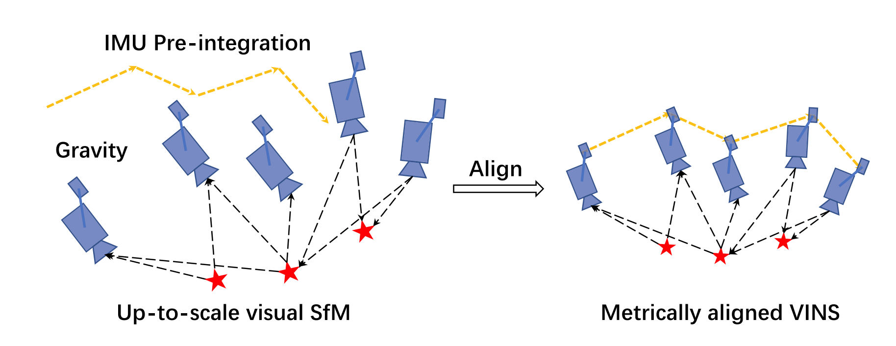
위 그림과 같이, 기본 아이디어는 up-to-scale visual structure와 IMU pre-integration을 맞추는 것입니다.

Gyroscope Bias Calibration

연속된 프레임 $b_k, b_{k+1}$ 이 있을때, 이전 과정(Visual SfM)으로부터 rotation $\mathbf {q}^{c_0}_{b_k}, \mathbf {q}^{c_0}_{b_{k+1}}$ 과 IMU preintegration으로부터 relative constraint $\hat{\boldsymbol{\gamma}}_{b{k+1}}^{b_k}$ 을 알 수 있습니다. 우리는 IMU preintegration term을 gyroscope bias에 따라 linearize하고, 다음에 나오는 cost function을 minimize 합니다.

\begin{equation} \begin{aligned} \min _{\delta b_\omega} \sum _{k \in \mathcal {B}} \left\Vert {\mathbf {q}^{c_0}_{b_{k+1}}}^{-1} \otimes \mathbf {q}^{c_0}_{b_{k}} \otimes \boldsymbol{\gamma }^{b_k}_{b_{k+1}} \right\Vert ^2 \\ \boldsymbol{\gamma }^{b_k}_{b_{k+1}} \approx \hat{\boldsymbol{\gamma }}^{b_k}_{b_{k+1}} \otimes {\left[\begin{array}{c}1\\ \frac{1}{2} \mathbf {J}^\gamma _{b_\omega} \delta \mathbf {b}_\omega \end{array}\right]} \end{aligned} \end{equation}

$\mathcal{B}$ 는 window에 있는 모든 frame들의 index

이를 통해 gyroscope bias의 initial calibration 값인 $\mathbf{b}_\omega$ 를 얻을 수 있습니다. 이 gyroscope bias를 이용하여 IMU preintegration terms $\hat{\boldsymbol{\alpha}}_{b_{k+1}}^{b_k}, \hat{\boldsymbol{\beta}}_{b_{k+1}}^{b_k}, \hat{\boldsymbol{\gamma}}_{b_{k+1}}^{b_k}$ 를 repropagate 합니다.

Velocity, Gravity Vector, and Metric Scale Initialization

gyroscope bias를 initialize한 후, navigation을 위한 essential state들인 velocity, gravity vector, and metric scale을 initialize 합니다.

\begin{equation} \begin{split} \mathcal {X}_{I} &= \left[ \mathbf {v}^{b_0}_{b_0},\,\mathbf {v}^{b_1}_{b_1},\, \ldots \,\mathbf {v}^{b_n}_{b_n},\,\mathbf {g}^{c_0},\, s \right] \end{split} \end{equation}

$\mathbf {v}^{b_k}_{b_k}$ : $k$ th 이미지에서의 velocity in the body frame

$\mathbf {g}^{c_0}$ : the gravity vector in the $c_0$ frame

$s$ : scales the monocular SfM to metric units

연속된 프레임 $b_k, b_{k+1}$ 이 있을때, 다음과 같은 식을 얻을 수 있습니다.

\begin{equation} \begin{aligned} {\boldsymbol{\alpha }}^{b_k}_{b_{k+1}} &= \mathbf {R}^{b_k}_{c_0} (s(\bar{\mathbf {p}}^{c_0}_{b_{k+1}} - \bar{\mathbf {p}}^{c_0}_{b_k}) + \frac{1}{2} \mathbf {g}^{c_0} {\Delta t}_k^2 - \mathbf {R}^{c_0}_{b_k} \mathbf {v}^{b_k}_{b_k}{\Delta t}_k) \\ {\boldsymbol{\beta }}^{b_k}_{b_{k+1}} &= \mathbf {R}^{b_k}_{c_0} (\mathbf {R}^{c_0}_{b_{k+1}}\mathbf {v}^{b_{k+1}}_{b_{k+1}} + \mathbf {g}^{c_0} {\Delta t}_k - \mathbf {R}^{c_0}_{b_k}\mathbf {v}^{b_k}_{b_{k}}). \end{aligned} \end{equation}

아래 링크의 (14)번 식 참조 IMU Preintegration

(6)과 (9)의 식을 결합하여 다음과 같은 linear measurement model이 나옵니다.

\begin{equation} \hat{\mathbf {z}}^{b_k}_{b_{k+1}} = {\left[\begin{array}{c}\hat{\boldsymbol{\alpha }}^{b_k}_{b_{k+1}} - \mathbf {p}^b_c + \mathbf {R}^{b_k}_{c_{0}}\mathbf {R}^{c_0}_{b_{k+1}}\mathbf {p}^b_c\\ \hat{\boldsymbol{\beta }}^{b_k}_{b_{k+1}} \end{array}\right]} = \mathbf {H}^{b_k}_{b_{k+1}} \mathcal {X}_I + \mathbf {n}^{b_k}_{b_{k+1}} \end{equation}

where

\begin{equation} \mathbf {H}^{b_k}_{b_{k+1}}= {\left[\begin{array}{cccc}-\mathbf {I}{\Delta t}_k &\mathbf {0} & \frac{1}{2}\mathbf {R}^{b_k}_{c_0} {\Delta t}_k^2 & \mathbf {R}^{b_k}_{c_0}(\bar{\mathbf {p}}^{c_0}_{c_{k+1}}-\bar{\mathbf {p}}^{c_0}_{c_k})\\ -\mathbf {I} &\mathbf {R}^{b_k}_{c_0}\mathbf {R}^{c_0}_{b_{k+1}} & \mathbf {R}^{b_k}_{c_0} {\Delta t}_k & \mathbf {0} \end{array}\right]} . \end{equation}

up-to-scale monocular visual SfM으로부터 우리는 $\mathbf{R}_{b_k}^{c_0}, \mathbf{R}_{b_{k+1}}^{c_0}, \bar{\mathbf{p}}_{c_k}^{c_0}, \bar{\mathbf{p}}_{c_{k+1}}^{c_0}$ 값을 얻을 수 있습니다. $\Delta t_k$ 는 연속된 두 프레임 사이의 time interval 입니다.

아래의 least-square problem을 풀어서 모든 frame에서의 body frame velocity, visual reference frame $(\cdot)^{c_0}$ 에서의 gravity vector, scale parameter를 얻을 수 있습니다.

\begin{equation} \begin{split} \min _{\mathcal {X}_I}\sum _{k \in \mathcal {B}} \left\Vert \hat{\mathbf {z}}^{b_k}_{b_{k+1}} - \mathbf {H}^{b_k}_{b_{k+1}} \mathcal {X}_I\right\Vert ^2 \end{split} \end{equation}

Gravity Refinement

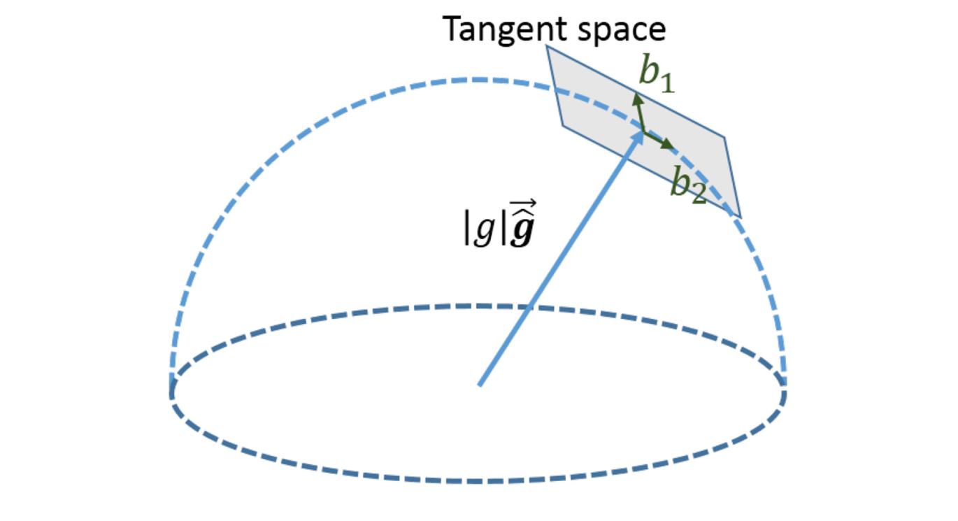
이전 과정에서 얻은 gravity vector는 magnitude를 제한하여 refine될 수 있습니다. 대부분의 경우에서 gravity vector의 magnitude는 알려져 있습니다. 결과적으로 gravity vector에 대한 2-DOF만 남게 됩니다. 따라서 2-DOF를 유지하면서 gravity를 tangent space위에 2개의 변수로 perturb합니다. gravity vector is perturbed by $g(\hat{\bar{\mathbf{g}}} + \delta\mathbf{g}), \delta\mathbf{g} = w_1\mathbf{b}_1 + w_2\mathbf{b}_2$ ( $g$ 는 알려진 magnitude of gravity, $\hat{\bar{\mathbf{g}}}$ 는 중력의 방향을 가리키는 unit vector). $\mathbf{b}_1, \mathbf{b}_2$ 는 tangent plane을 spanning하는 직교하는 basis 입니다. $w_1, w_2$ 는 $\mathbf{b}_1, \mathbf{b}_2$ 에 대한 2D perturbation 입니다. 우리는 tangent space 위에서 임의의 $\mathbf{b}_1, \mathbf{b}_2$ 를 찾을 수 있습니다. 그리고 (9)에 $g(\hat{\bar{\mathbf{g}}} + \delta\mathbf{g})$ 를 대입하고, 다른 변수와 함께 2D $\delta \mathbf{g}$ 를 풉니다. 이 과정을 $\hat{\mathbf{g}}$ 이 수렴할 때까지 반복합니다.

Completing Initialization

위의 과정 이후 중력을 z축 방향 rotate하는 방법으로 world frame과 camera frame $c_0$ 간의 rotate $\mathbf {q}_{c_0}^{w}$ 를 얻을 수 있습니다. 그리고 모든 변수들을 reference frame $(\cdot)^{c_0}$ 에서 world frame $(\cdot)^{w}$ 으로 변환합니다. body frame의 veloocity또한 world frame으로 rotate 됩니다. visual SfM을 통해 구한 Translational components들은 metric unit으로 scale 됩니다. Initialize 과정이 끝나고 tightly coupled monocular VIO로 이 모든 metric value들이 공급됩니다.