VINS-Mono 논문 번역 & 공부 (2)

2022. 1. 21.

#SLAM #VINS-Mono

이전에 쓴 글 이후 Section.VIII Experimental Result 전까지 내용을 정리하였습니다.
코드 Github 논문 PDF

Introduction

VINS-Mono는 다음과 같은 특징을 가지고 있습니다.

robust initialization procedure that is able to bootstrap the system from unknown initial states.
tightly coupled, optimization-based monocular VIO with camera–IMU extrinsic calibration and IMU bias correction.
online relocalization and four degrees-of-freedom (DOF) global pose graph optimization.
pose graph reuse that can save, load, and merge multiple local pose graphs.

Overview

Structure

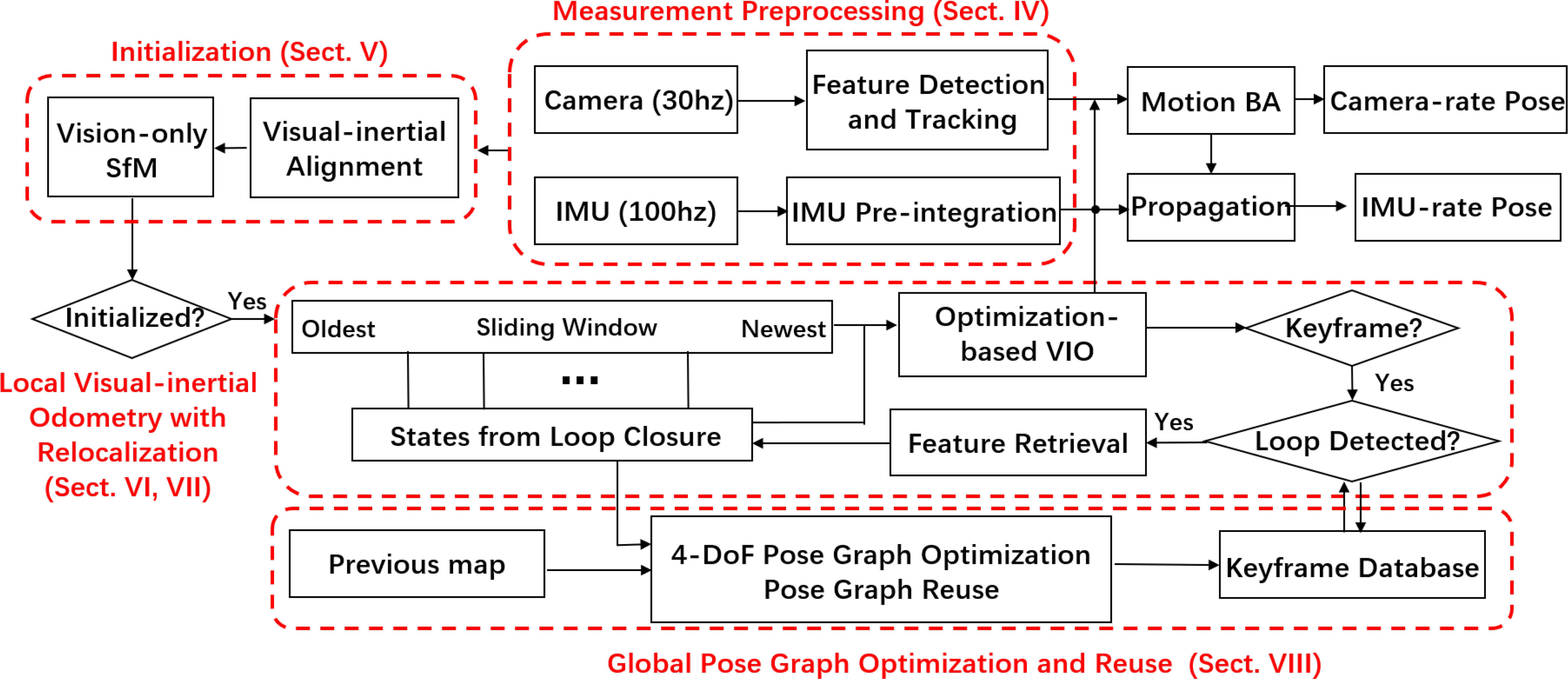
monocular visual-inertial state estimator의 구조입니다.

시스템은 measurement preprocessing으로 시작합니다. (Section IV)

feature가 extract and tracked되고, 두 프레임 사이의 IMU 측정값이 preintergrate 됩니다.

Initialization 과정은 필요한 모든 값들을 제공합니다. (Section V)

for bootstrapping the subsequent nonlinear optimization-based VIO.
pose, velocity, gravity vector, gyroscope bias, and three-dimensional (3-D) feature location.

The VIO (Section VI) with relocalization (Section VII) 모듈

preintegrated IMU measurements와 feature observations를 tightly 통합합니다.

마지막으로 pose graph optimization 모듈. (Section VIII)

takes in geometrically verified relocalization results.
perform global optimization to eliminate the drift.
also achieves the pose graph reuse.

The VIO와 pose graph optimization 모듈은 각각의 thread에서 동시에 동작합니다.

Notation and Frame Definitions

$(\cdot)^w$ : world frame, 중력의 방향은 world frame의 z축과 align되어 있습니다.
$(\cdot)^b$ : body frame (IMU frame)
$(\cdot)^c$ : camera frame
$\mathbf{R}$ : rotation matrix
$\mathbf{q}$ : Hamilton quaternion
- 주로 state vector에 사용
- 3D vector의 편한 회전 연산을 위해서 사용됨
$\mathbf{q}_{b}^{w}, \mathbf{p}_{b}^{w}$ : rotation and translation from the body frame to the world frame
$b_k$ : the body frame while taking the $k$ th image
$c_k$ : the camera frame while taking the $k$ th image.
$\otimes$ : represents the multiplication operation between two quaternions
$\mathbf{g}^w = [0,0,g]^T$ : the gravity vector in the world frame
$\hat{(\cdot)}$ : the noisy measurement or estimation of a certain quantity

Tightly Coupled Monocular VIO

estimator를 initialization한 후에 높은 정확도와 robust한 state estimation을 위한 sliding window-based tightly coupled monocular VIO를 수행합니다.

Formulation

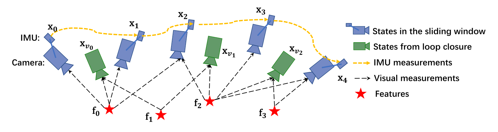
sliding window의 full state vector는 다음과 같이 정의됩니다.

\begin{equation} \begin{aligned} \mathcal {X} &= \left[ \mathbf {x}_0,\,\mathbf {x}_{1},\, \ldots \,\mathbf {x}_{n},\, \mathbf {x}^b_c,\, \lambda _0,\,\lambda _{1},\, \ldots \,\lambda _{m} \right] \\ \mathbf {x}_k &= \left[ \mathbf {p}^w_{b_k},\,\mathbf {v}^w_{b_k},\,\mathbf {q}^w_{b_k}, \,\mathbf {b}_a, \,\mathbf {b}_g \right], k\in [0,n] \\ \mathbf {x}^b_c &= \left[ \mathbf {p}^b_c,\,\mathbf {q}^b_{c} \right] \tag{13} \end{aligned} \end{equation}

$\mathbf {x}_k$ : $k$ th image가 capture되었을 때의 IMU state (world frame에서의 position, velocity, and orientation과 body frame에서의 acceleration bias and gyroscope bias를 포함)

$n$ : the total number of keyframes

$m$ : is the total number of features in the sliding window.

$\lambda_l$ : the inverse distance of the $l$ th feature from its first observation.

visual-inertial bundle adjustment formulation을 사용합니다. maximum posteriori estimation을 위해서 모든 측정값의 residuals의 prior와 Mahalanobis norm의 합을 다음과 같이 minimize합니다.

\begin{equation} \min _{\mathcal {X}} \left\lbrace \left\Vert \mathbf {r}_p - \mathbf {H}_p \mathcal {X} \right\Vert ^2 + \sum _{k \in \mathcal {B}} \left\Vert \mathbf {r}_{\mathcal {B}}(\hat{\mathbf {z}}^{b_k}_{b_{k+1}},\, \mathcal {X}) \right\Vert _{\mathbf {P}^{b_k}_{b_{k+1}}}^2 \right. \left. + \sum _{(l,j) \in \mathcal {C}} \rho (\left\Vert \mathbf {r}_{\mathcal {C}}(\hat{\mathbf {z}}^{c_j}_l, \, \mathcal {X}) \right\Vert _{\mathbf {P}^{c_j}_l}^2) \right\rbrace \tag{14} \end{equation}

where the Huber norm[37] is defined as

\begin{equation} \rho (s)=\left\{\begin{array}{ll}s & s \leq 1\\ 2\sqrt{s}-1 & s > 1. \end{array}\right. \end{equation} \tag{15}

$\mathbf {r}_{\mathcal {B}}(\hat{\mathbf {z}}^{b_k}_{b_{k+1}},\, \mathcal {X})$ : residuals for IMU measurements

$\mathbf {r}_{\mathcal {C}}(\hat{\mathbf {z}}^{c_j}_l, \, \mathcal {X})$ : residuals for visual measurements

residual terms에 대한 좀더 자세한 정의는 바로 뒤에서 나옵니다. (Sections VI-B and VI-C)

$\mathcal{B}$ : set of all IMU measurements

$\mathcal{C}$ : set of features that have been observed at least twice in the current sliding window. $\{\mathbf{r}_p , \mathbf{H}_p\}$ : prior information from marginalization.

The Ceres solver [38] is used for solving this nonlinear problem.

[37]

[38]

IMU Measurement Residual

sliding window 안에 있는 연속된 $b_k$ 와 $b_{k+1}$ frame의 IMU 측정값에서 preintegrate된 IMU 측정값의 residual은 다음과 같이 정의됩니다.

\begin{equation} \begin{split} & \mathbf {r}_{\mathcal {B}}(\hat{\mathbf {z}}^{b_k}_{b_{k+1}},\, \mathcal {X})= {\left[\begin{array}{c}\delta \boldsymbol{\alpha }^{b_k}_{b_{k+1}}\\ \delta \boldsymbol{\beta }^{b_k}_{b_{k+1}}\\ \delta \boldsymbol{\theta }^{b_k}_{b_{k+1}}\\ \delta {\mathbf {b}_a}\\ \delta {\mathbf {b}_g}\\ \end{array}\right]}\\ &={\left[\begin{array}{c}\mathbf {R}^{b_k}_{w}(\mathbf {p}^{w}_{b_{k+1}} - \mathbf {p}^{w}_{b_k} + \frac{1}{2}\mathbf {g}^{w} \Delta t_k^2 - \mathbf {v}^{w}_{b_k} \Delta t_k) -\boldsymbol{\hat{\alpha }}^{b_k}_{b_{k+1}} \\ \mathbf {R}^{b_k}_{w}(\mathbf {v}^{w}_{b_{k+1}} + \mathbf {g}^{w} \Delta t_k- \mathbf {v}^{w}_{b_k})- \boldsymbol{\hat{\beta }}^{b_k}_{b_{k+1}} \\ 2{\left[\begin{array}{c}\mathbf {q}^{w^{-1}}_{b_{k}} \otimes \mathbf {q}^{w}_{b_{k+1}} \otimes {(\hat{\boldsymbol{\gamma }}^{b_k}_{b_{k+1}})}^{-1} \end{array}\right]}_{xyz}\\ {\mathbf {b}_a}_{b_{k+1}} - {\mathbf {b}_a}_{b_k}\\ {\mathbf {b}_w}_{b_{k+1}} - {\mathbf {b}_w}_{b_k} \end{array}\right]} \end{split} \tag{16} \end{equation}

$[\cdot]_{xyz}$ 는 error-state를 표현하는 quaternion $\mathbf{q}$ 에 대하여 vector부분의 성분만 추출한 것 입니다. $\delta\boldsymbol\theta_{b_{k+1}}^{b_k}$ 는 3-D error-state representation of quaternion. $[\hat{\boldsymbol{\alpha}}^{b_k}_{b{k+1}}, \hat{\boldsymbol{\beta}}^{b_k}_{b{k+1}}, \hat{\boldsymbol{\gamma}}^{b_k}_{b{k+1}}]$ 는 두 이미지 프레임 사이의 preintegrate된 IMU 측정값이다. Accelerometer와 gyroscope biases또한 실시간 correction을 위해 residual식에 포함되어있습니다. $i$ 번째 이미지에서 처음 관찰된 $l$ 번째의 feature가 있을 때 $j$ 번째 이미지에서 관측된 feature과의 residual은 다음과 같이 정의됩니다.

Visual Measurement Residual

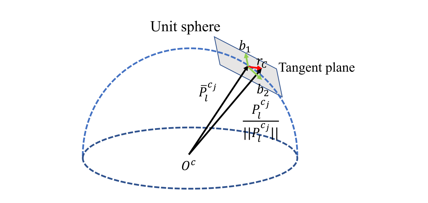
generalized image plane에서의 reprojection error를 정의하는 전통적인 핀홀 카메라 모델과 다르게, 우리는 unit sphere에서의 카메라 측정값 residual을 정의합니다. 대부분 카메라의 optics는 unit sphere의 표면을 연결하는 unit ray로 modeling할 수 있습니다.

\begin{equation} \begin{aligned} &\mathbf {r}_{\mathcal {C}}(\hat{\mathbf {z}}^{c_j}_l,\, \mathcal {X}) = {\left[\begin{array}{c}\mathbf {b}_1 \ \ \mathbf {b}_2 \end{array}\right]}^T \cdot \left({\hat{\bar{\mathcal {P}}}^{c_j}_l} - \frac{\mathcal {P}^{c_j}_l}{\Vert \mathcal {P}^{c_j}_l\Vert }\right) \\ &\hat{\bar{\mathcal {P}}}^{c_j}_l = {\pi _c}^{-1} \left({\left[\begin{array}{c}\hat{u}^{c_j}_l \\ \hat{v}^{c_j}_l \end{array}\right]} \right) \\ &\mathcal {P}^{c_j}_l = \mathbf {R}^c_b \Bigg(\mathbf {R}^{b_j}_w \Bigg(\mathbf {R}^w_{b_i} \Bigg(\mathbf {R}^b_c \frac{1}{\lambda _l} {\pi _c}^{-1} \left({\left[\begin{array}{c}\hat{u}^{c_i}_l \\ \hat{v}^{c_i}_l \end{array}\right]} \right) + \mathbf {p}^b_c \Bigg) + \mathbf {p}^w_{b_i} - \mathbf {p}^w_{b_j}\Bigg) - \mathbf {p}^b_c\Bigg) \tag{17} \end{aligned} \end{equation}

$[\hat{u}_l^{c_i}, \hat{v}_l^{c_i}]$ : $i$ 번째 이미지에서 처음으로 관찰된 $l$ 번째의 feature

$[\hat{u}_l^{c_j}, \hat{v}_l^{c_j}]$ : $j$ 번째 이미지에서 관찰된 같은 feature $π_c^{−1}$ : 카메라 intrinsic parameter를 이용해 pixel의 위치를 unit vector로 변환하는 back projection function

vision residual는 2-DOF이기 때문에 우리는 residual vector를 tangent plane위 project합니다. $\mathbf {b}_1, \mathbf {b}_2$ 는 $\hat{\bar{\mathcal {P}}}^{c_j}_l$ 를 span하는 임의의 직교 bases입니다. 식 (14)에서 사용된 variance $\mathbf {P}^{c_j}_l$ 또한 픽셀좌표계에서 unit sphere로 propagate됩니다.

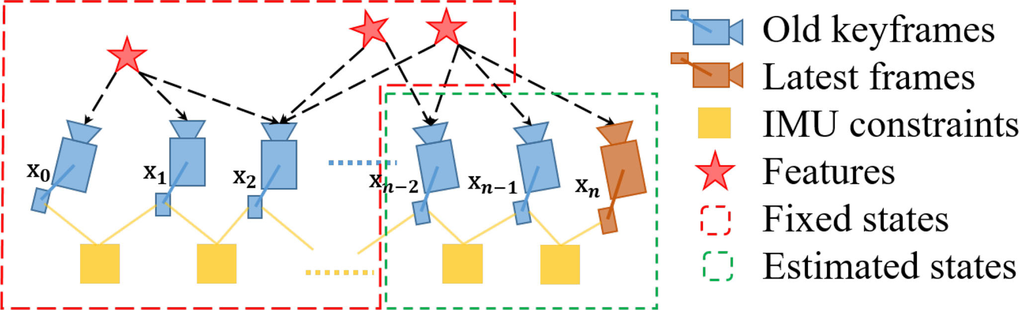
Marginalization

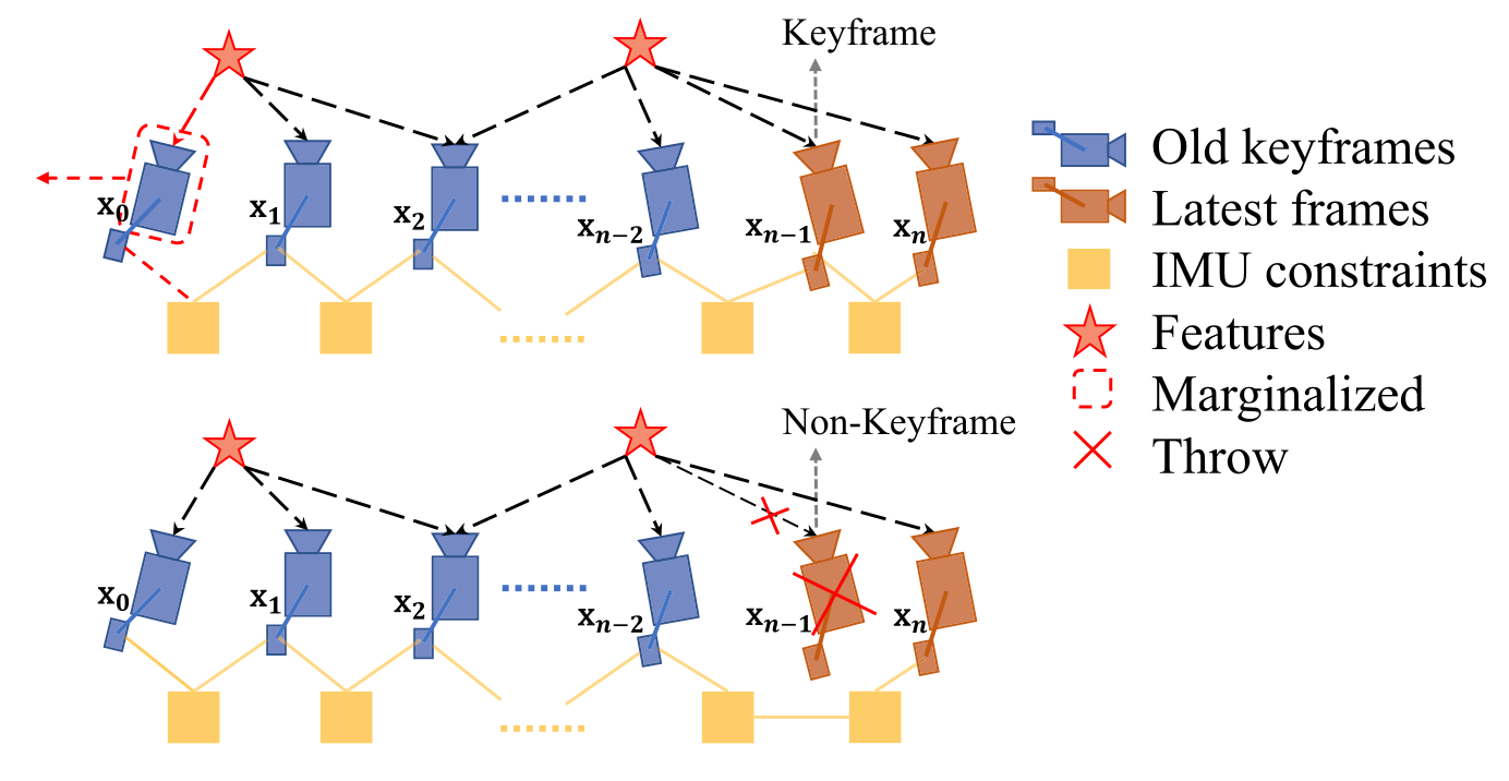
optimization-based VIO 계산이 너무 복잡해지는 것을 막기위해 marginalization을 수행합니다. IMU state $\mathbf x_k$ 와 feature $\lambda_l$ 을 선택적으로 marginalize out하면서 marginalized state에 따른 측정값을 prior로 convert 합니다.

위의 그림에서 보이는 것처럼 마지막에서 2번째 프레임이 keyframe이라면 그 프레임은 윈도우안에 유지되고, 가장 오래된 프레임과 해당하는 측정값이 marginalized out됩니다. 만약 keyframe이 아니라면 visual 측정값은 던져버리고 IMU측정값만 keep합니다. 우리는 시스템의 sparsity를 유지하기 위해 nonkeyframe의 측정값을 marginalize out하지 않습니다. marginalization scheme의 목적은 공간적으로 분리된 keyframe을 유지하는 것입니다. 이것은 feature traiangulation을 위한 충분한 parallex를 가지고 있다는 확신으 주고, large excitation에서 accelerometer 측정값을 유지하는 가능성을 maximize 합니다.

marginalization은 Schur complement[39]을 이용해 수행됩니다. 우리는 삭제된 state와 관련된 모든 marginalized measurements에 기반하여 새로운 prior를 생성합니다. 새로운 prior는 이미 존재하는 prior에 더해집니다.

[39]

marginalization결과는 linearizaion에서 early fix되기 때문에 최적의 결과가 아닐 수도 있습니다. 그러나 VIO에서 작은 drifting이 허용되기 때문에 marginalization에서 초래되는 부정적인 결과는 치명적이지 않다고 주장합니다.

Motion-Only Visual-Inertial Optimization for Camera-Rate State Estimation

컴퓨팅 파워가 부족한 디바이스에서는 nonlinear 최적화의 계산이 복잡해 camera rate보다 계산속도가 나오지 않아서 tightly coupled monocular VIO가 수행될 수 없습니다. 우리는 이를 위해서 state estimation이 camera rate(30Hz)으로 동작할 수 있도록 가벼운 motion-only visual-inertial optimization을 사용합니다.

motion-only visual-inertial optimization의 cost function은 식 (14)와 같습니다. 그러나 sliding window의 모든 state를 optimize하는 대신 오직 마지막에서부터 정해진 숫자의 IMU state(pose, velocity)를 optimize합니다. feature depth, extrinsic parameters, bias, and old IMU states 등의 optimize를 하지 않는 값들을 상수로 봅니다. 모든 visual 측정값과 IMU측정값을 이용합니다. 결과는 single-frame PnP방법봅다 훨신 smooth한 state를 얻을 수 있습니다. 이것은 drone이나 AR application활용에 강점을 가지는 low-latency camera-rate pose estimation을 가능하게 합니다.

IMU Forward Propagation for IMU-Rate State Estimation

IMU measurements는 visual보다 훨씬 빠른 rate으로 값이 들어옵니다. VIO의 frequency가 image capture frequency에 의해 제한되지만, 마지막 estimate된 VIO값을 최근의 IMU측정값을 이용해 IMU-rate으로 propagate할 수 있습니다. high-frequency state estimate은 closed-loop closure의 state feedback으로 활용될 수 있습니다. 섹션 IX-C에서 활용을 볼 수 있습니다.

Relocalization

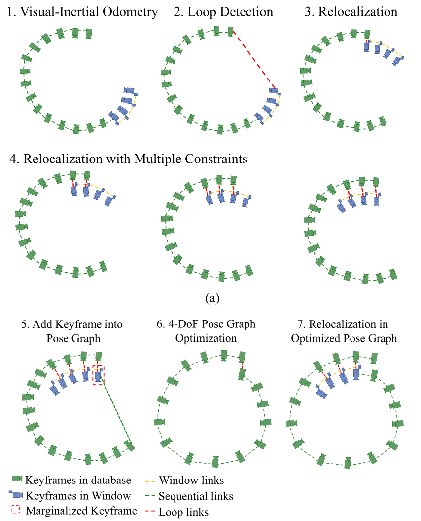
sliding window와 marginalization scheme은 계산의 복잡도를 낮춰주지만 누적되는 오차(drift)를 만들게됩니다. drift를 제거하기 위해 monocular VIO와 원할하게 통합되는 tightly coupled relocalization module이 사용됩니다.

relocalization과정은 이미 방문했던 위치를 감지하는 loopdetection module로 시작합니다. 그 다음으로 loop-clusre 후보와 현재 프레임간의 feature-level connection이 생성됩니다. 이 feature 연결은 monocular VIO module에 tightly integrate되어 결과적으로 minimum compuatation으로 drift-free state estimate을 가능하게 합니다. multiple feature들의 multiple observation은 relocalization에 directly 사용되어 결과적으로 높은 정확도와 더 좋은 state estimation smoothness를 가지게 됩니다.

Loop Detection

우리는 loop detection을 위해 DBoW2[29](state-of-the-art bag-of-words place recognition approach)를 활용합니다. monocular VIO에 사용되는 corner feature외에도 500개보다 더 많은 corner가 BRIEF descriptor[40]에 의해 detect되고 describe됩니다.

[29]

[40]

추가적인 corner feature는 더 좋은 loop detection recall rate을 위해 사용됩니다. descriptor는 visual database를 query하기 위한 visual word로 간주됩니다. DBoW2는 시간, 공간적 consistency를 확인한 후 loop-closure 후보를 return 합니다. 우리는 feature 검색을 위한 모든 BRIEF descriptor를 유지하지만메모리 유지를 위해 raw 이미지는 무시합니다.

Feature Retrieval

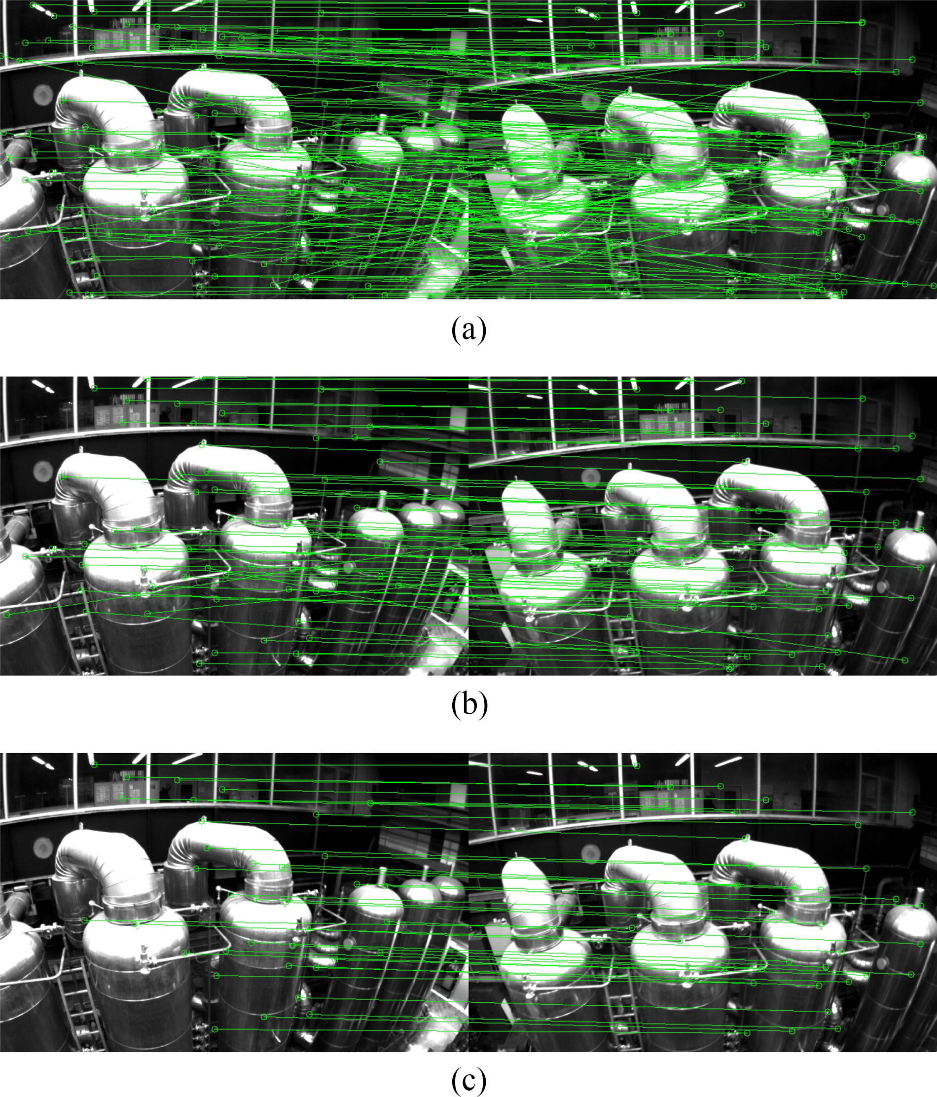
loop가 detect 되었을 때, feature 검색을 통해 loop-closure 후보와 local sliding window 사이의 connection이 생깁니다. BRIEF descriptor matching을 통해 공통점이 찾아집니다. Descriptor matching은 잘못된 pair를 만들 수도 있기 때문에 우리는 마지막에 2 step outlier제거 과정을 진행합니다.

2-D–2-D
- RANSAC[33]을 이용한 기본 matrix 테스트
- 테스트를 수행하기 위해 우리는 현재 이미지와 loop-closure 후보 이미지에서 검색된 feature의 2D 위치을 이용합니다.
3D–2-D
- RANSAC[35]을 이용한 PnP 테스트.
- 알고있는 local sliding window의 feature가 있는 3D위치와 loop-closure 후보 이미지의 2D위치를 바탕으로 PnP테스트를 수행합니다.

outlier 제거를 한 후 우리는 loop detection을 후보가 아니라 맞다고 취급하고, relocalization을 수행합니다.

Tightly Coupled Relocalization

relocalization 과정은 효과적으로 현재 sliding window와 과거의 pose를 align 합니다. relocalization을 하는 동안 우리는 모든 loop-closure 프레임들의 pose를 상수로 취급합니다. 모든 IMU 측정값, visual 측정값, 검색된 feature의 공통점을 같이 이용하여 sliding window를 optimize합니다. 우리는 VIO안에서의 visual 측정값과 같은 loop-closure frame $v$ 와 검색된 feature를 위한 visual 측정값의 model을 식 (17)과 같이 쉽게 쓸수 있습니다. 단지 다른점은 pose graph나 과거의 odometry output에서 직접 구한 loop-closure frame의 pose $(\hat{\mathbf q}_v^w, \hat{\mathbf p}_v^w)$ 를 상수로 사용하는 것입니다. 마지막으로 우리는 식 (14)의 nonlinear cost function을 약간 수정하고 loop term을 더하여 다음의 식을 얻을 수 있습니다.

\begin{equation} \begin{aligned} \min _{\mathcal {X}} \left\lbrace \left\Vert \mathbf {r}_p - \mathbf {H}_p \mathcal {X} \right\Vert ^2 + \sum _{k \in \mathcal {B}} \left\Vert \mathbf {r}_{\mathcal {B}}(\hat{\mathbf {z}}^{b_k}_{b_{k+1}}, \mathcal {X}) \right\Vert _{\mathbf {P}^{b_k}_{b_{k+1}}}^2 \right. \left. + \sum _{(l,j) \in \mathcal {C}} \rho (\left\Vert \mathbf {r}_{\mathcal {C}}(\hat{\mathbf {z}}^{c_j}_l, \mathcal {X}) \right\Vert _{\mathbf {P}^{c_j}_l}^2) \right. \\ \left. + \underbrace{ {\sum} _{(l,v) \in \mathcal {L}} \rho (\left\Vert \mathbf {r}_{\mathcal {C}}(\hat{\mathbf {z}}^{v}_l, \mathcal {X}, \hat{\mathbf {q}}^w_v, \hat{\mathbf {p}}^w_v) \right\Vert _{\mathbf {P}^{c_v}_l}^2) }_{\text{reprojection error in the loop-closure frame}} \right\rbrace \tag{18} \end{aligned} \end{equation}

$\mathcal{L}$ : loop-closure 프레임에서 검색된 feature observation set

$(l, v)$ : loop-closure frame $v$ 에서 찾은 $l$ 번째 feature

cost function은 식 (14)와 약간 다르지만 loop-closure frames의 pose가 상수취급되기 때문에 풀어야하는 문제의 dimension은 똑같습니다. 만약에 현재 sliding window에서 loop closure가 여러개 생긴다면 우리는 loop-closure feature와 동시에 대응하는 모든 frame에 대해 optimize를 수행합니다. 이는 relocalization을 위한 multiview 제한을 만들고, 더 높은 정확도와 부드러운 결과를 가져옵니다. relocalization이후 일관성 유지를 위한 global optimization이 수행됩니다(in Section VIII).

Global Pose Graph Optimization And Map Reuse

relocalization이후 globally consistent configuration에 과거의 pose를 추가할 수 있도록 추가적인 pose graph optimization이 수행됩니다.

Four Accumulated Drift Direction

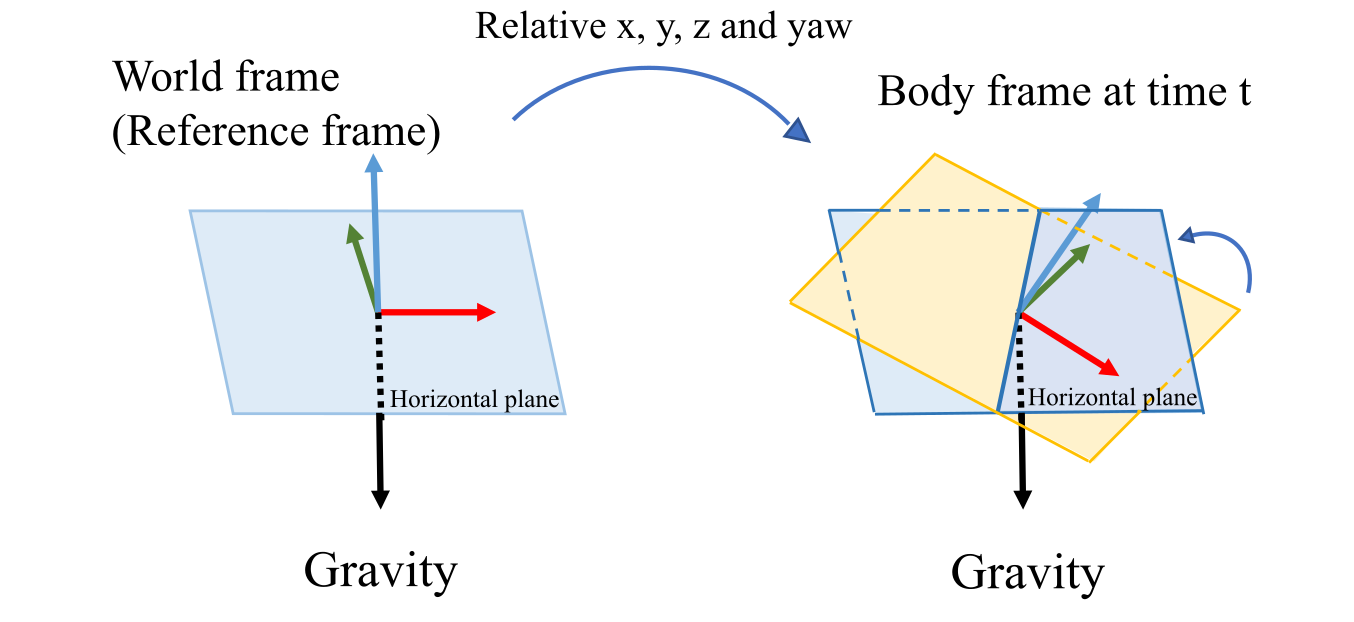
중력 측정값으로부터 우리는 이득을 얻는데, 그것은 roll과 pitch를 완전히 관측할 수 있는 것입니다. 위의 그림처럼 object의 움직임과 함께, 3D position과 rotation은 reference frame을 기준을 바뀝니다. 그러나 우리는 horizontal plane을 중력 vector를 통해 찾을 수 있습니다. 이것은 항상 우리가 absolute한 roll과 pitch 각도를 구할 수 있음을 의미합니다. 따라서 roll과 pitch는 world frame에서 absolute합니다. 그에 비해 $x, y, z$ 와 yaw는 reference frame을 기준삼아 상대적으로 estimate 됩니다. 누적되는 drift는 오직 $x, y, z$ 와 yaw에서 발생됩니다. valid한 정보와 drift를 효과적으로 보정하기위해 우히는 drift가 생기지 않는 roll과 pitch를 fix시키고 나머지 4DoF pose graph optimization을 수행합니다.

Adding Keyframes Into the Pose Graph

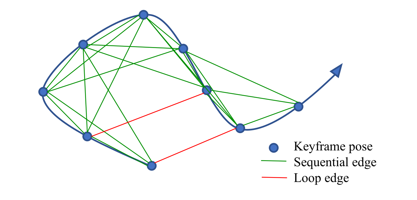
keyframe은 VIO 과정 이후 pose graph에 더해집니다. 모든 keyfraem은 pose graph에서 vertex로 간주됩니다. vertex와 vertex 사이는 위 그림처럼 2개의 edge로 연결됩니다.

Sequential Edge

keyframe은 과거의 keyframe과 여러개의 sequential edge를 만들어냅니다. sequential edge는 상대적인 VIO에서 직접바로 구해지는 두 keyframe간의 상대적인 transformation을 표현합니다. keyframe $i$ 와 과거의 keyframe $j$ 가 있을 때 sequential edge 상대적인 position $\hat{\mathbf{p}}^i_{ij}$ 과 yaw angle $\hat{\psi}_{ij}$ 를 가지고 있습니다.

\begin{equation} \begin{aligned} \hat{\mathbf {p}}^i_{ij} =& {\hat{\mathbf {R}}}_{i}^{{w}^{-1}}(\hat{\mathbf {p}}^w_j - \hat{\mathbf {p}}^w_i) \\ \hat{\psi }_{ij} =& \hat{{\psi }}_{j} - \hat{\psi }_{i}. \tag{19} \end{aligned} \end{equation}

Loop-Closure Edge

만약에 keyframe이 loop connection을 가지고 있다면 이것은 loop-closure frame을 연결합니다. 마찬가지로 loop-closure edge또한 식(19)와 같이 상대적인 위치의 4DoF를 가집니다. loop-closure edge의 값은 relocalization의 결과로 얻어집니다.

4-DOF Pose Graph Optimization

우리는 frame $i$ 와 $j$ 사이 edge의 residual을 간단하게 다음과 같이 정의합니다.

\begin{equation} \begin{split} \mathbf {r}_{i,j}(\mathbf {p}^w_i, \psi _i, \mathbf {p}^w_j, \psi _j)= {\left[\begin{array}{c}\mathbf {R}(\hat{\phi }_i,\hat{\theta }_i,\psi _i)^{-1} (\mathbf {p}^w_j - \mathbf {p}^w_i)-\hat{\mathbf {p}}^i_{ij}\\ \psi _j - \psi _i - \hat{\psi }_{ij}\\ \end{array}\right]} \end{split} \tag{20} \end{equation}

$\hat{\phi }_i,\hat{\theta }_i$ 는 monocular VIO를 통해 구한 fix되어 estimate한 roll, pitch각도입니다.

모든 graph의 sequential edge와 loop closure edge는 다음의 cost function을 minimize하여 optimize됩니다.

\begin{equation} \begin{aligned} \min _{\mathbf {p}, \psi } \left\lbrace \sum _{(i,j) \in \mathcal {S}} \left\Vert \mathbf {r}_{i,j} \right\Vert ^2 + \sum _{(i,j) \in \mathcal {L}} \rho (\left\Vert \mathbf {r}_{i,j} \right\Vert ^2) \right\rbrace \end{aligned} \tag{21} \end{equation}

$\mathcal{S}$ : 모든 sequential edge set

$\mathcal{L}$ : 모든 loop-closure edge set

tightly coupled relocalization과정이 이미 잘못구한 loop closure를 지우지만, 우리는 또 다른 Huber norm $\rho(\cdot)$ 을 추가하여 혹시나 발생할 수 있는 잘못된 loop의 영향을 줄입니다. 반대로 우리는 이미 충분히 outlier를 제거하는 과정을 포함하는 VIO에서 edge를 구하기 때문에 sequential edge를 위한 robust norm을 사용하지 않습니다.

Pose Graph Merging

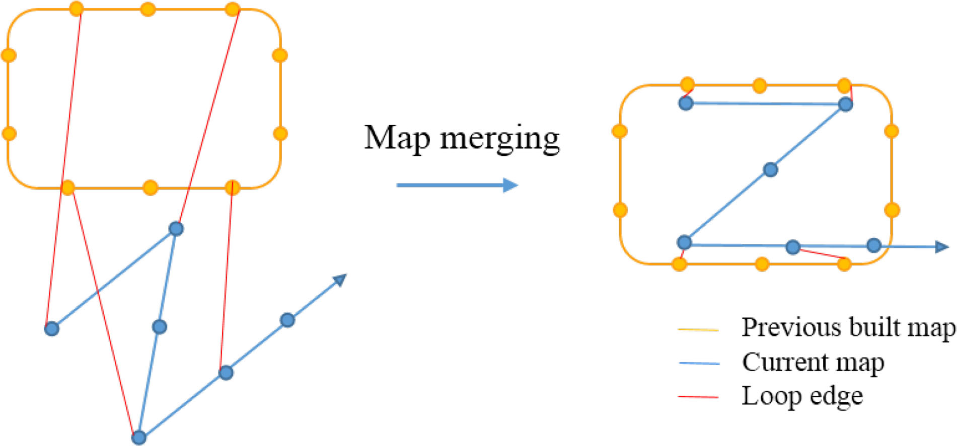
pose graph은 현재 map만 optimize하는 것이 아니라 과거에 만들어진 map과 현재 map을 merge 합니다. 만약 우리가 예전에 만든 map을 load하고 두 map 사이의 loop connection을 발견한다면 우리는 둘을 merge 합니다. 모든 edge가 상대적인 제한을 주기 때문에 pose graph optimization은 loop connection을 하면서 자동적으로 두 map을 merge 합니다. 위 그림에서 보이는 것 처럼 loop edge에 의해 현재 map이 과거의 map으로 당겨집니다. 모든 vertex와 edge는 상대적인 변수입니다. 따라서 우리는 단지 pose graph의 첫번째 vertex만 fix하면 됩니다.

Pose Graph Saving

우리 pose graph의 구조는 매우 간단합니다. 우리는 keyframe(vetex)의 descriptor를 포함하여 vertex와 edge만 저장하면 됩니다. raw 이미지는 메모리를 고려하여 무시됩니다. $i$ 번째의 keyframe을 저장하기위한 state는 다음과 같습니다.

\begin{equation} [i, \hat{\mathbf {p}}^w_i,\hat{\mathbf {q}}^w_i, v, \hat{\mathbf {p}}^i_{iv}, \hat{\psi }_{iv}, \mathbf {D}(u,v,\text{des})] \tag{22} \end{equation}

$i$ : frame index

$\hat{\mathbf p}_i^w, \hat{\mathbf q}_i^w$ : position and orientation from VIO

$v$ : loop-closure frame’s index (If this frame has a loopclosure frame)

$\hat{\mathbf{p}}^i_{ij}, \hat{\psi}_{ij}$ : relative position and yaw angle between these two frames, which is obtained from relocalization.

$\mathbf {D}(u,v,\text{des})$ : the feature set. Each feature contains 2-D location and its BRIEF descriptor

Pose Graph Loading

우리는 keyframe을 load하기 위해 저장하는 format과 똑같은 format을 사용합니다. 모든 keyframe은 pose graph에서 vertex입니다. vetex의 initial pose는 $\hat{\mathbf p}_i^w, \hat{\mathbf q}_i^w$ 입니다. loop edge는 loop information인 $\hat{\mathbf{p}}^i_{ij}, \hat{\psi}_{ij}$ 에 의해 직접 생성됩니다. 모든 keyframe은 식 (19)처럼 이웃한 keyframe과 몇몇개의 sequential edges를 생성합니다. pose graph를 loading한 후 우리는 global 4DoF pose graph 바로 한번 수행합니다. pose graph의 저장과 loading은 pose graph의 사이즈와 linear한 관계입니다.