Visual Odometry Tutorial Part 2

2022. 1. 4.

#SLAM

Matching, Robustness, Optimization, and Application

레퍼런스들은 여기서 확인 가능 PDF

Feature Selection and Matching

There are two main approaches to find feature points and their correspondences.

find features in one image and track them in the following images using local search techniques
- more suitable when the images are taken from nearby viewpoints
independently detect features in all the images and match them based on some similarity metric between their descriptors
- more suitable when a large motion or viewpoint change is expected

Early research in VO is opted for the former approach [2]–[5]

early works were conceived for small-scale environments, where images were taken from nearby viewpoints

Last decade concentrated on the latter approach [1], [6]–[9]

focus has shifted to large-scale environments
the images are taken as far apart as possible from each to limit the motion-drift-related issues.The SURF detector builds upon the SIFT but uses box filters to approximate the Gaussian, resulting in a faster computation compared to SIFT, which is achieved with integral images

Feature Detection

During the feature-detection step, the image is searched for salient keypoints that are likely to match well in other images.

local feature : an image pattern that differs from its immediate neighborhood in terms of intensity, color, and texture.

For VO, point detectors, such as corners or blobs, are important

because their position in the image can be measured accurately.

A corner is defined as a point at the intersection of two or more edges.

A blob is an image pattern that differs from its immediate neighborhood in terms of intensity, color, and texture.

The appealing properties that a good feature detector should have are

localization accuracy (both in position and scale)
repeatability (i.e., a large number of features should be redetected in the next images)
computational efficiency
robustness (to noise, compression artifacts, blur)
distinctiveness (so that features can be accurately matched across different images)
invariance [to both photometric (e.g., illumination) and geometric changes (rotation, scale, perspective distortion)]

The VO literature is characterized by many point-feature detectors

such as corner detectors (e.g., Moravec [2], Forstner [10], Harris [11], Shi-Tomasi [12], and FAST [13]) and blob detectors (SIFT [14], SURF [15], and CENSURE [16])

overview of these detectors can be found in [17]

Each detector has its own pros and cons.

Corner detectors
- fast to compute but are less distinctive,
- better localized in image position than blobs
- less localized in scale than blobs
- corners cannot be redetected as often as blobs after large changes in scale and viewpoint
Blob detectors
- more distinctive but slower to detect.
- blobs are not always the right choice in some environments
  - for instance, SIFT automatically neglects corners that urban environments are extremely rich of

For these reasons, the choice of the appropriate feature detector should be carefully considered

depending on the

computational constraints

real-time requirements

environment type

motion baseline (i.e., how nearby images are taken).

	Corner Detector	Blob Detector	Rotation Invariant	Scale Invatiant	Affine Invariant	Repeatability	Localization Accuracy	Robustness	Efficiency
Harris	o		o			+++	+++	++	++
Shi-Tomasi	o		o			+++	+++	++	++
FAST	o		o	o		++	++	++	++++
SIFT		o	o	o	o	+++	++	+++	+
SURF		o	o	o	o	+++	++	++	++
CENSURE		o	o	o	o	+++	++	+++	+++

Notice that SIFT, SURF, and CENSURE are not true affine invariant detectors but were empirically found to be invariant up to certain changes of the viewpoint.

A performance evaluation of feature detectors and descriptors for indoor VO has been given in [18] and for outdoor environments in [9] and [19].

Every feature detector consists of two stages

apply a feature-response function on the entire image
such as the corner response function in the Harris detector or the difference-of-Gaussian (DoG) operator of the SIFT.
apply nonmaxima suppression on the output of the first step.

The goal is to identify all local minima (or maxima) of the feature-response function. The output of the nonmaxima suppression represents detected features.

additional The trick to make a detector invariant to scale changes consists in applying the detector at lower-scale and upper-scale versions of the same image. Invariance to perspective changes is instead attained by approximating the perspective distortion as an affine one. SIFT is a feature devised for object and place recogntion and found to give outstanding results for VO. The SURF detector builds upon the SIFT but uses box filters to approximate the Gaussian, resulting in a faster computation compared to SIFT, which is achieved with integral images.

Feature Descriptor

In the feature description step, the region around each detected feature is converted into a compact descriptor that can be matched against other descriptors.

The simplest descriptor of a feature is its appearance, that is, the intensity of the pixels in a patch around the feature point.

In this case, error metrics such as the sum of squared differences (SSDs) or the normalized cross correlation (NCC) can be used to compare intensities [20].
Contrary to SSD, NCC compensates well for slight brightness changes.
An alternative and more robust image similarity measure is the Census transform [21]
- converts each image patch into a binary vector representing which neighbors have their intensity above or below the intensity of the central pixel.
- The patch similarity is then measured through Hamming distance.

In many cases, the local appearance of the feature is not a good descriptor.

because its appearance will change with orientation, scale, and viewpoint changes.
In fact, SSD and NCC are not invariant to any of these changes, and, therefore, their use is limited to images taken at nearby positions.

One of the most popular descriptors for point features is the SIFT.

process
- basically a histogram of local gradient orientations.
- The patch around the feature is decomposed into a 4 X 4 grid.
- For each quadrant, a histogram of eight gradient orientations is built.
- All these histograms are then con catenated together, forming a 128-element descriptor vector.
- To reduce the effect of illumination changes, the descriptor is then normalized to unit length.
stable against changes in illumination, rotation, and scale, and even up to 60° changes in viewpoint.
can, in general, be computed quadratic in the number of features, which can become for corner or blob features
- however, its performance will decrease on corners.
- corner descriptor won’t be as distinctive as for blobs, which, conversely, lie in highly textured regions of the image.

Between 2010 and 2011, three new descriptors have been devised, which are much faster to compute than SIFT an SURF

A simple binary descriptor named BRIEF [22]
- it uses pairwise brightness comparisons sampled from a patch around the keypoint.
- extremely fast to extract and compare
- exhibits high discriminative power in the absence of rotation and scale change.
ORB [23] was Inspired by BRIEF
- tackles orientation invariance and an optimization of the sampling scheme for the brightness value pairs.
BRISK [24]
- keypoint detector based on FAST, which allows scale and rotation invariance
- a binary descriptor that uses a configurable sampling pattern.

Feature Matching

The feature-matching step searches for corresponding features in other images.

The simplest way for matching features between two images is to compare all feature descriptors in the first image to all other feature descriptors in the second image.

Descriptors are compared using a similarity measure.

If the descriptor is the local appearance of the feature, then a good measure is the SSD or NCC.

For SIFT descriptors, this is the Euclidean distance.

Mutual Consistency Check

After comparing, the best correspondence of a feature in the second image is chosen as that with the closest descriptor (in terms of distance or similarity)

this stage may result with features in the second image matching with more than one feature in the first image.

To decide which match to accept, the mutual consistency check can be used.

Only pairs of corresponding features that mutually have each other as a preferred match are accepted as correct.

Constrained Matching

A disadvantage of this exhaustive matching is that it is quadratic in the number of features, which can become impractical when the number of features is large (e.g., several thousands).

A better approach is to use an indexing structure to rapidly search for features near a given feature.

such as a multidimensional search tree or a hash table

A faster feature matching is to search for potential correspondences in regions of the second image where they are expected to be.

These regions can be predicted using a motion model and the three-dimensional (3-D) feature position (if available).
The motion can be given by an additional sensor, or can be inferred from the previous position assuming a constant velocity model, as proposed in [26].
sensor like IMU, wheel odometry [25], laser, and GPS.
The predicted region is then calculated as an error ellipse from the uncertainty of the motion and that of the 3-D point.

Alternatively, if only the motion model is known but not the 3-D feature position, the corresponding match can be searched along the epipolar line in the second image.

This process is called epipolar matching.
a single 2-D feature and the two camera centers define a plane in the 3-D space that intersect both images into two lines, called epipolar lines.
An epipolar line can be computed directly from a 2-D feature and the relative motion of the camera, as explained in Part I of this tutorial.
Each feature in the first image has a different epipolar line in the second image.

In stereovision, instead of computing the epipolar line for each candidate feature, the images are usually rectified.

Image rectification is a remapping of an image pair into a new image pair where epipolar lines of the left and right images are horizontal and aligned to each other.
This has the advantage of facilitating image-correspondence search
since epipolar lines no longer have to be computed for each feature: the correspondent of one feature in the left (right) image can be searched across those features in the right (left) image, which lie on the same row. Image rectification can be executed efficiently on graphics processing units (GPUs).
In stereovision, the relative position between the two cameras is known precisely.
However, if the motion is affected by uncertainty, the epipolar search is usually expanded to a rectangular area within a certain distance from the epipolar line.
In stereovision, SSD, NCC, and Census transform are the widely used similarity metrics for epipolar matching [91].

Feature Tracking

An alternative is to detect features in the first image and, then, search for their corresponding matches in the following images.

This detect-then-track approach is suitable for VO applications where images are taken at nearby locations, where the amount of motion and appearance deformation between adjacent frames is small.
For this particular application, SSD and NCC can work well.
if features are tracked over long image sequences, their appearance can undergo larger changes.
- a solution is to apply an affine-distortion model to each feature.
The resulting tracker is often called KanadeLucasTomasi (KLT) tracker

Discussion

SIFT Matching

For SIFT feature matching, a distance-ratio test was proposed by the authors initially, for use in place and object detection [14].

This distance-ratio test accepts the closest match (the one with minimum Euclidean distance) only if the ratio between the closest and the second closest match is smaller than a user-specified threshold.
The idea behind this test is to remove matches that might be ambiguous, e.g., due to repetitive structure.
The threshold for the test can only be set heuristically and an unlucky guess might remove correct matches as well.

Therefore, in many cases, it might be beneficial to skip the ratio test and let RANSAC take care of the outliers as explained in the “Outlier Removal” section.

Lines and Edgelets

An alternative to point features for VO is to use lines or edgelets, as proposed in [27] and [28].

can be used in addition to points in structured environments
may provide additional cues.
such as direction (of the line or edgelet), and planarity and orthogonality constraints.
Contrary to points, lines are more difficult to match.
- because lines are more likely to be occluded than points.
- the origin and end of a line segment of edgelet may not exist (e.g., occlusions and horizon line).

Number of Features and Distribution

The distribution of the features in the image has been found to affect the VO results remarkably [1], [9], [29].

In particular, more features provide more stable motion-estimation results than with fewer features.

But at the same time, the keypoints should cover the image as evenly as possible.

To do this, the image can be partitioned into a grid, and the feature detector is applied to each cell by tuning the detection thresholds until a minimum number of features are found in each subimage [1].
As a rule of the thumb, 1,000 features is a good number for a 640 X 480-pixel image.

Dense and Correspondence-Free Methods

An alternative to sparse-feature extraction is to use dense methods.

such as optical flow [30], or feature-less methods [31].

Optical flow
- aims at tracking, ideally, each individual pixel or a subset of the whole image (e.g., all pixels on a grid specified by the user).
- similar to feature tracking, it assumes small motion between frames.
- and, therefore, is not suitable for VO applications since motion error accumulates quickly.
feature-less motion-estimation methods

such as [31]: all the pixels in the two images are used to compute the relative motion using a harmonic Fourier transform.
- This method has the advantage to work especially with low-texture images.
- computationally extremely expensive (can take up to several minutes).
- recovered motion is less accurate than with feature-based methods.

Outlier Removal

Matched points are usually contaminated by outliers, that is, wrong data associations.

Possible causes of outliers

image noise

occlusions

blur

changes in viewpoint and illumination for which the mathematical model of the feature detector or descriptor does not account for.

For the camera motion to be estimated accurately, it is important that outliers be removed.

Outlier rejection is the most delicate task in VO.

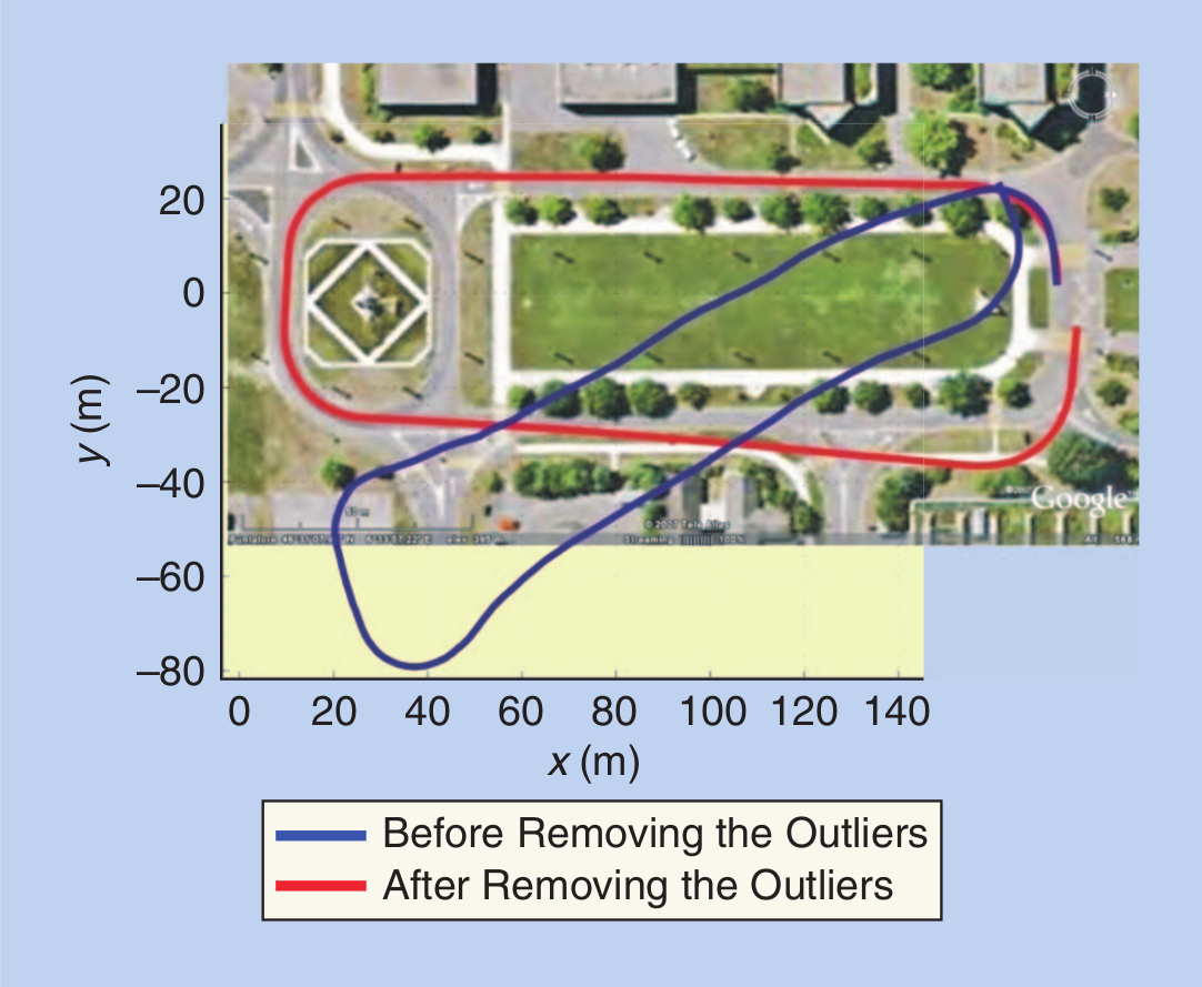
RANSAC

The solution to outlier removal consists in taking advantage of the geometric constraints introduced by the motion model. Robust estimation methods, such as M-estimation [32], case deletion, and explicitly fitting and removing outliers [33], can be used but these often work only if there are relatively few outliers.

RANSAC [34] has been established as the standard method for model estimation in the presence of outliers.

The idea behind RANSAC is to compute model hypotheses from randomly sampled sets of data points and then verify these hypotheses on the other data points.
The hypothesis that shows the highest consensus with the other data is selected as a solution.
For two-view motion estimation as used in VO
- the estimated model is the relative motion $(R,\ t)$ between the two camera positions
- the data points are the candidate feature correspondences.
Inlier points to a hypothesis are found by computing the point-to-epipolar line distance [35].
- The point-to-epipolar line distance is usually computed as a first-order approximation—called Sampson distance—for efficiency reasons [35].
- An alternative to the point-to-epipolar line distance is the directional error proposed by Oliensis [36].
  - The directional error measures the angle between the ray of the image feature and the epipolar plane.
  - The authors claim that the use of the directional error is advantageous for the case of omnidirectional and wide-angle cameras but also beneficial for the standard camera case.

The outline of RANSAC is given in Algorithm 1.

Algorithm 1. VO from 2-D-to-2-D correspondences.
1. Initial: let A be a set of N feature correspondences
2. Repeat
  1. Randomly select a sample of s points from A
  2. Fit a model to these points
  3. Compute the distance of all other points to this model
  4. Construct the inlier set (i.e. count the number of points whose distance from the model $< d$ )
  5. Store these inliers
  6. Until maximum number of iterations reached
3. The set with the maximum number of inliers is chosen as a solution to the problem
4. Estimate the model using all the inliers.

The number of subsets (iterations) N that is necessary to guarantee that a correct solution is found can be computed by

\begin{equation} N = \frac{\log(1-p)}{\log(1-(1-\epsilon)^s)}, \end{equation}

$s$ is the number of data points from which the model can be instantiated

$\epsilon$ is the percentage of outliers in the data points

$p$ is the requested probability of success [34].

For the sake of robustness, in many practical implementations, N is usually multiplied by a factor of ten.

More advanced implementations of RANSAC estimate the fraction of inliers adaptively, iteration after iteration.

As observed, RANSAC is a probabilistic method and is nondeterministic in that it exhibits a different solution on different runs; however, the solution tends to be stable when the number of iterations grows.

Minimal Model Parameterizations

As can be observed in Figure 7, $N$ is exponential in the number of data point $s$ necessary to estimate the model.

Therefore, there is a high interest in using a minimal parameterization of the model.

In Part I of this tutorial, an eight-point minimal solver for uncalibrated cameras was described.
- Although it works also for calibrated cameras, the eight-point algorithm fails when the scene points are coplanar.
when the camera is calibrated, its 6 DoF motion can be inferred from a minimum of five-point correspondences
- and the first solution to this problem was given in 1913 by Kruppa [37].
- Several five-point minimal solvers were proposed later in [38]–[40], but an efficient implementation, based on [39], was found only in 2003 by Nister [41] and later revised in [42].
  - Before that, the six- [43], seven- [44], or eight- solvers were commonly used.
- However, the five-point solver has the advantage that it works also for planar scenes.

Despite the five-point algorithm represents the minimal solver for 6 DoF motion of calibrated cameras, in the last few decades, there have been several attempts to exploit different cues to reduce the number of motion parameters.

In [49], Fraundorfer et al. proposed a three-point minimal solver for the case of two known camera-orientation angles.
- For instance, this can be used when the camera is rigidly attached to a gravity sensor (in fact, the gravity vector fixes two camera-orientation angles).
Later, Naroditsky et al. [50] improved on that work by showing that the three-point minimal solver can be used in a four-point (three-plus-one) RANSAC scheme.
- The three-plus-one stands for the fact that an additional far scene point (ideally, a point at infinity) is used to fix the two orientation angles.
A two-point minimal solver for 6-DoF VO was proposed by Kneip et al. [51], which uses the full rotation matrix from an IMU rigidly attached to the camera.

In the case of planar motion, the motion model complexity is reduced to 3 DoF and can be parameterized with two points as described in [52].

For wheeled vehicles, Scaramuzza et al. [9], [53] showed that the motion can be locally described as planar and circular, and, therefore, the motion model complexity is reduced to 2 DoF, leading to a one-point minimal solver.
Using a single point for motion estimation is the lowest motion parameterization possible and results in the most efficient RANSAC algorithm.
Additionally, they show that, by using histogram, voting outliers can be found in a small, single iteration.

A performance evaluation of five-, two-, and one-point RANSAC algorithms for VO was finally presented in [54].

To recap, the reader should remember that, if the camera motion is unconstrained, the minimum number of points to estimate the motion is five, and, therefore, the five-point RANSAC (or the six-, seven-, or eight-point one) should be used.

Table 1. Number of RANSAC iterations.

Number of points (s) 8 7 6 5 4 2 1
Number of iterations (N) 1,177 587 292 145 71 16 7
These values were obtained from (1)
- assuming a probability of success $P = 99\%$
- assuming a percentage of outliers $\epsilon = 50\%$

Number of points (s)	8	7	6	5	4	2	1
Number of iterations (N)	1,177	587	292	145	71	16	7

Reducing the Iterations of RANSAC

As can be observed in Table 1, the five-point RANSAC requires a minimum of 145 iterations. However, in reality, the things are not always so straightforward.

Sometimes, the number of outliers is underestimated and using more iterations increases the chances to find more inliers.
In some cases, it can even be necessary to allow for thousands of iterations.

Because of this, several works have been produced in the endeavor of increasing the speed of RANSAC.

The maximum likelihood estimation sample consensus [55] makes the measurement of correspondences more reliable and improves the estimate of the hypotheses.
The progressive sample consensus [56] ranks the correspondences based on their similarity and generates motion hypotheses starting from points with higher rank.
Preemptive RANSAC [57] uses preemptive scoring of the motion hypotheses and a fixed number of iterations.
Uncertainty RANSAC [58] incorporates feature uncertainty and shows that this determines a decrease in the number of potential outliers, thus enforcing a reduction in the number of iterations.
In [59], a deterministic RANSAC approach is proposed, which also estimates the probability that a match is correct.

What all the mentioned algorithms have in common is that the motion hypotheses are directly generated from the points.

Conversely, other algorithms operate by sampling the hypotheses from a proposal distribution of the vehicle motion model [60], [61].

Among all these algorithms, preemptive RANSAC has been the most popular one because the number of iterations can be fixed a priority, which has several advantages when real-time operation is necessary.

Is It Really Better to Use a Minimal Set in RANSAC?

If one is concerned with certain speed requirements, using a minimal point set is definitely better than using a nonminimal set.

However, even the five-point RANSAC might not be the best idea if the image correspondences are very noisy.

In this case, using more points than a minimal set is proved to give better performance (in terms of accuracy and number of inliers) [62], [63].

To understand it, consider a single iteration of the five-point RANSAC:

at first, five random points are selected and used to estimate the motion model;
second, this motion hypothesis is tested on all other points.
select five points or more points
1. If the selected five points are inliers with large image noise
  - the motion estimated from them will be inaccurate
  - will exhibit fewer inliers when tested on all the other points.
2. if the motion is estimated from more than five points using the five-point solver
  - the effects of noise are averaged
  - the estimated model will be more accurate
  - with the effect that more inliers will be identified.

Therefore, when the computational time is not a real concern and one deals with noisy features, using a nonminimal set may be better than using a minimal set [62].

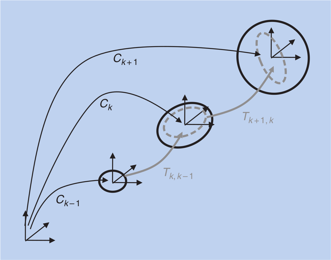
Error Propagation

In VO, individual transformations $T_{k, k-1}$ are concatenated to form the current pose of the robot $C_k$ (see Part I of this tutorial).

Each of these transformations $T_{k, k-1}$ has an uncertainty, and the uncertainty of the camera pose $C_k$ depends on the uncertainty of past transformations.

The uncertainty of the transformation $T_{k+1, k}$ computed by VO depends on camera geometry and the image features

A derivation for the stereo case can be found in [3].

In the following, the uncertainty propagation is discussed.

Each camera pose $C_k$ and each transformation $T_{k, k-1}$ can be represented by a six-element vector containing the position $(x, y, z)$ and orientation (in Euler angles $\phi, \theta, \psi$ ).

These six-element vectors are denoted by $\vec{C}_{k}$ and $\vec{T}_{k,k-1}$ , respectively, e.g., $\vec{C}_k = (x, y, z, \phi, \theta, \psi)^\top$ .

Each transformation $\vec{T}_{k,k-1}$ is represented by its mean and covariance $\Sigma_{k,k-1}$ .

The covariance matrix $\Sigma_{k,k-1}$ is a 6 X 6 matrix.

The camera pose $\vec{C_k}$ is written as $\vec{C}_{k} = f(\vec{C}_{k-1}, \vec{T}_{k,k-1})$ , that is a function of the previous pose $\vec{C}_{k-1}$ and the transformation $\vec{T}_{k,k-1}$ with their covariances $\Sigma_{k-1}$ and $\Sigma_{k,k-1}$ , respectively.

The combined covariance matrix $\vec{C_k}$ is a 12 X 12 matrix and a compound of the covariance matrices and $\Sigma_{k,k-1}$ and $\Sigma_{k-1}$ .

$\vec{C_k}$ can be computed by using the error propagation law [64], which uses a first-order Taylor approximation; therefore,

\begin{align} \Sigma_{k} &= J\begin{bmatrix} \Sigma_{k-1} & 0 \\ 0 & \Sigma_{k,k-1} \end{bmatrix}J^\top \\ &= J_{\vec{C}_{k-1}}\Sigma_{k-1}{J_{\vec{C}_{k-1}}}^\top + J_{\vec{T}_{k,k-1}}\Sigma_{k,k-1}{J_{\vec{T}_{k,k-1}}}^\top, \end{align}

Where $J_{\vec{C}_{k-1}}$ , $J_{\vec{T}_{k,k-1}}$ are the Jacobians of f with respect to $\vec{C}_{k-1}$ and $\vec{T}_{k,k-1}$ , respectively.

As can be observed from this equation, the camera-pose uncertainty is always increasing when concatenating transformations. Thus, it is important to keep the uncertainties of the individual transformations small to reduce the drift.

Camera Pose Optimization

VO computes the camera poses by concatenating the transformations, in most cases from two subsequent views at times $k$ and $k-1$ (see Part I of this tutorial).

However, it might also be possible to compute transformations between the current time $k$ and the $n$ last time steps $T_{k,k-2}, ..., T_{k,k-n}$ , or even for any time step $T_{i,j}$ .

If these transformations are known, they can be used to improve the camera poses by using them as additional constraints in a pose-graph optimization.

Pose-Graph Optimization

The camera poses computed from VO can be represented as a pose graph

pose graph : where the camera poses are the nodes and the rigid-body transformations between the camera poses are the edges between nodes [65].

Each additional transformation that is known can be added as an edge into the pose graph. The edge constraints $e_{ij}$ define the following cost function:

\begin{equation} \sum_{e_{ij}}{\|C_i-T_{e_{ij}}C_j\|}^2, \end{equation}

where $T_{e_{ij}}$ is the transformation between the poses $i$ and $j$ .

Pose graph optimization seeks the camera pose parameters that minimize this cost function.

The rotation part of the transformation makes the cost function nonlinear, and a nonlinear optimization algorithm (e.g., Levenberg-Marquardt) has to be used.

Loop Constraints for Pose-Graph Optimization

Loop constraints are valuable constraints for pose graph optimization.

These constraints form graph edges between nodes that are usually far apart and between which large drift might have been accumulated.

Commonly, events like reobserving a landmark after not seeing it for a long time or coming back to a previously mapped area are called loop detections [66].
Loop constraints can be found by evaluating visual similarity between the current camera images and past camera images.
Visual similarity can be computed using global image descriptors (e.g., [67] and [68]) or local image descriptors (e.g., [69]).

Recently, loop detection by visual similarity using local image descriptors got a lot of attention and one of the most successful methods are based on the so-called visual words [70]–[73].

In these approaches, an image is represented by a bag of visual words.
The visual similarity between two images is then computed as the distance of the visual word histograms of the two images.
The visual word-based approach is extremely efficient to compute visual similarities between large sets of image data, a property important for loop detection.
A visual word represents a high-dimensional feature descriptor (e.g., SIFT or SURF) with a single integer number.
- For this quantization, the original high-dimensional descriptor space is divided into non-overlapping cells by k-means clustering [74], which is called the visual vocabulary.
- All feature descriptors that fall within the same cell will get the cell number assigned, which represents the visual word.
Visual-word-based similarity computation is often accelerated by organizing the visual-word database as an inverted-file data structure [75] that makes use of the finite range of visual vocabulary.
Visual similarity computation is the first step of loop detection.
After finding the top-n similar images, usually a geometric verification using the epipolar constraint is performed
- for confirmed matches, a rigid-body transformation is computed using wide-baseline feature matches between the two images.
- This rigid-body transformation is added to the pose graph as an additional loop constraint.

Windowed (or Local) Bundle Adjustment

Windowed bundle adjustment [76] is similar to pose-graph optimization as it tries to optimize the camera parameters but, in addition, it also optimizes the 3-D landmark parameters at the same time.

It is applicable to the cases where image features are tracked over more than two frames.

Windowed bundle adjustment considers a so-called window of $n$ image frames and then performs a parameter optimization of camera poses and 3-D landmarks for this set of image frames.

In bundle adjustment, the error function to minimize is the image reprojection error:

\begin{equation} \arg\min_{X^i, C_k}\sum_{i,k}{\|p^i_k-g(X^i,C_k)\|}^2, \end{equation}

where $p^i_k$ is the $i$ th image point of the 3-D landmark $X^i$ measured in the $k$ th image

$g(X^i,C_k)$ is its image reprojection according to the current camera pose $C_k$ .

The reprojection error is a nonlinear function, and the optimization is usually carried out using Levenberg-Marquardt.

This requires an initialization that is close to the minimum. Usually, a standard two-view VO solution serves as initialization.

The Jacobian for this optimization problem has a specific structure that can be exploited for efficient computation [76].

Windowed bundle adjustment reduces the drift compared to two-view VO

because it uses feature measurements over more than two image frames.
The current camera pose is linked via the 3-D landmark, and the image feature tracks not only the previous camera pose but also the camera poses further back.

The current and $n-1$ previous camera poses need to be consistent with the measurements over $n$ image frames.

The choice of the window size $n$ is mostly governed by computational reasons.

The computational complexity of bundle adjustment in general is $O((qM+lN)^3)$
$M$ : number of points

$N$ : number of cameras poses

$q$ : number of parameters for points

$l$ : number of parameters for camera poses.
A small window size limits the number of parameters for the optimization and thus makes real-time bundle adjustment possible.

It is possible to reduce the computational complexity by just optimizing over the camera parameters and keeping the 3-D landmarks fixed, e.g., if the 3-D landmarks are accurately triangulated from a stereo setup.

Applications

VO has been successfully applied within various fields.

Table 2. Software and data sets.

Author	Description	Link
Willow Garage	OpenCV: A computer vision library maintained by Willow Garage. The library includes many of the feature detectors mentioned in this tutorial (e.g., Harris, KLT, SIFT, SURF, FAST, BRIEF, ORB). In addition, the library contains the basic motion-estimation algorithms as well as stereo-matching algorithms.	http://opencv.willowgarage.com
Willow Garage	Robot operating system (ROS): A huge library and middleware maintained by Willow Garage for developing robot applications. Contains a VO package and many other computer-vision-related packages.	http://www.ros.org
Willow Garage	Point cloud library (PCL): A 3-D-data-processing library maintained from Willow Garage, which includes useful algorithms to compute transformations between 3-D-point clouds.	http://pointclouds.org
Henrik Stewenius et al.	Five-point algorithm: An implementation of the five-point algorithm for computing the essential matrix.	http://www.vis.uky.edu/~stewe/FIVEPOINT/
Changchang Wu et al.	SiftGPU: Real-time implementation of SIFT.	http://cs.unc.edu/~ccwu/siftgpu
Nico Cornelis et al.	GPUSurf: Real-time implementation of SURF.	http://homes.esat.kuleuven.be/~ncorneli/gpusurf
Christopfer Zach	GPU-KLT: Real-time implementation of the KLT tracker.	http://www.inf.ethz.ch/personal/chzach/opensource.html
Edward Rosten	Original implementation of the FAST detector.	http://www.edwardrosten.com/work/fast.html
Michael Calonder	Original implementation of the BRIEF descriptor.	http://cvlab.epfl.ch/software/brief/
Leutenegger et al.	BRISK feature detector.	http://www.asl.ethz.ch/people/lestefan/personal/BRISK
Jean-Yves Bouguet	Camera Calibration Toolbox for MATLAB.	http://www.vision.caltech.edu/bouguetj/calib_doc
Davide Scaramuzza	OCamCalib: Omnidirectional Camera Calibration Toolbox for MATLAB.	https://sites.google.com/site/scarabotix/ocamcalib-toolbox
Christopher Mei	Omnidirectional camera calibration toolbox for MATLAB.	http://homepages.laas.fr/~cmei/index.php/Toolbox
Mark Cummins	Fast appearance-based mapping: Visual-word-based loop detection.	http://www.robots.ox.ac.uk/~mjc/Software.htm
Friedrich Fraundorfer	Vocsearch: Visual-word-based place recognition and image search.	http://www.inf.ethz.ch/personal/fraundof/page2.html
Manolis Lourakis	Sparse bundle adjustment (SBA)	http://www.ics.forth.gr/~lourakis/sba
Christopher Zach	Simple sparse bundle adjustment (SSBA)	http://www.inf.ethz.ch/personal/chzach/opensource.html
Rainer Kuemmerle et al.	G2O: Library for graph-based nonlinear function optimization. Contains several variants of SLAM and bundle adjustment.	http://openslam.org/g2o
RAWSEEDS EU Project	RAWSEEDS: Collection of data sets with different sensors (lidars, cameras, and IMUs) with ground truth.	http://www.rawseeds.org
SFLY EU Project	SFLY-MAV data set: Camera-IMU data set captured from an aerial vehicle with Vicon data for ground truth.	http://www.sfly.org
Davide Scaramuzza	ETH OMNI-VO: An omnidirectional-image data set captured from the roof of a car for several kilometers in a urban environment. MATLAB code for VO is provided.	http://sites.google.com/site/scarabotix

Conclusions

Part II of the tutorial has summarized the remaining building blocks of the VO pipeline:

how to detect and match salient and repeatable features across frames
robust estimation in the presence of outliers
bundle adjustment.
error propagation
applications
and links to publicly available code are included.

In the presence of loop closures, VO can be used as a building block for a complete SLAM algorithm to reduce motion drift.

Challenges that still remain are to develop and demonstrate large-scale and long-term implementations, such as driving autonomous cars for hundreds of miles.